1
since this page started loading...
💀
Incentive Alignment Bonds: Making Public Goods Financially and Politically Profitable
Government spending is optimized for lobbying intensity, not net societal value. Programs with 100:1 benefit-cost ratios get billions while programs with negative returns get hundreds of billions. Incentive Alignment Bonds flip this by creating a capital pool that rewards politicians (via campaign support and post-office opportunities) for funding high-NSV programs over low-NSV alternatives. The result: public good becomes private profit for both investors and elected officials.
Abstract
Government spending correlates with lobbying intensity, not marginal societal value. Programs with benefit-cost ratios exceeding 100:1 (vaccines, e-governance) receive single-digit billions while programs with negative net returns (military beyond deterrence, fossil fuel subsidies) receive hundreds of billions. This paper introduces Incentive Alignment Bonds (IABs), financial instruments that realign politician incentives with net societal value optimization. IABs create a capital pool that rewards politicians (via campaign support and post-office career opportunities) for funding high-NSV programs over low-NSV alternatives. The mechanism requires no legislative change: existing PAC infrastructure, impact bonds, and prediction markets can deploy it today. Analysis of a proposed 1% Treaty redirecting $27.2B/year from military spending to medical research shows expected returns exceeding 100:1 for early investors. The 90:1 capital asymmetry ($454T in household wealth vs. $5T for concentrated interests) means diffuse beneficiaries can outspend incumbent lobbies once coordination problems are solved. IABs solve that coordination problem by turning political change into an investable asset class.
Keywords
mechanism design, public choice, political economy, collective action, social impact bonds, campaign finance, incentive compatibility

The Problem in One Sentence: Politicians are rewarded for funding low-NSV programs (military beyond deterrence: 0.7:1 BCR) and punished for funding high-NSV programs (medical research: 100:1+ BCR) because concentrated interests outlobby diffuse beneficiaries, so government spending is optimized for lobbying intensity rather than marginal societal value.
The Solution: Incentive Alignment Bonds (IABs) flip the incentives by creating a capital pool that rewards politicians (with campaign support and post-office career opportunities) for funding high-NSV programs, making marginal societal value optimization the career-maximizing choice.
1 Introduction
1.1 The Information-Incentive Disconnect
A central puzzle in political economy is why policies with large positive net social welfare often fail to be adopted. The economic case for many global public goods, including climate mitigation, pandemic preparedness, and clinical trials, is overwhelming, yet governments don’t do them. The conventional diagnosis is wrong: the problem is not lack of information or resources, but wrong incentives.
Rankings of government programs by net societal value already exist and are systematically ignored. The Copenhagen Consensus has published rigorous benefit-cost ratio (BCR) analyses since 2004132. Their findings are clear: childhood vaccinations (101:1 BCR), e-government procurement (125:1), and maternal health interventions (87:1) dramatically outperform military spending beyond deterrence requirements (~0.7:1) and fossil fuel subsidies (negative net societal value). GiveWell, Open Philanthropy, the IMF, and numerous academic institutions produce similar analyses.
Yet government spending patterns have not shifted. The U.S. spends $16 on military operations for every $1 on diplomacy and humanitarian aid. Programs with benefit-cost ratios exceeding 100:1 receive single-digit billions while programs with negative net societal value receive hundreds of billions.
Here’s the reality: If a private equity firm allocated capital like the U.S. government, it would invest $100M in ventures that destroy $500M in value while rejecting ventures that return $10B. The firm would be bankrupt within a year. The government simply prints more money and calls it “fiscal policy.”
The marginal value of producing another ranking is zero. We don’t need more information. Politicians already know which programs produce net societal value. We need a mechanism to make existing information consequential in the political utility function (the mathematical representation of what politicians actually care about: reelection, money, status).
This paper argues that politicians maximize reelection probability, post-office career prospects, and status, not aggregate social welfare. The problem is not that decision-makers don’t know which programs produce value. They do know. They don’t care, because caring doesn’t appear in their utility function.
Mancur Olson’s seminal work The Logic of Collective Action133 established that groups with concentrated interests (small groups with huge per-person stakes, like military contractors) systematically outcompete groups with diffuse interests (millions of people with small individual stakes, like citizens who’d benefit from cures) in political competition. Why? A small group facing large per-member stakes will invest more in lobbying than a large group facing small per-member stakes. This holds even when total welfare losses exceed total welfare gains. The beneficiaries of inefficient policies (military contractors, pharmaceutical incumbents, fossil fuel producers) are concentrated. The beneficiaries of efficient policies (citizens who would benefit from cures, climate stability, reduced existential risk) are diffuse.
The result is a systematic distortion of democratic governance. The U.S. Constitution’s Preamble charges government to “promote the general Welfare,” the welfare of all citizens, not the welfare of any particular faction. Yet Olsonian dynamics ensure that government routinely promotes specific welfare (of concentrated interests who can afford to lobby) at the expense of general welfare (of the diffuse public). This is not corruption in the legal sense; it is the predictable equilibrium (stable outcome where nobody wants to change their behavior) of rational actors operating within existing institutional rules. The problem is not bad actors but bad incentives.
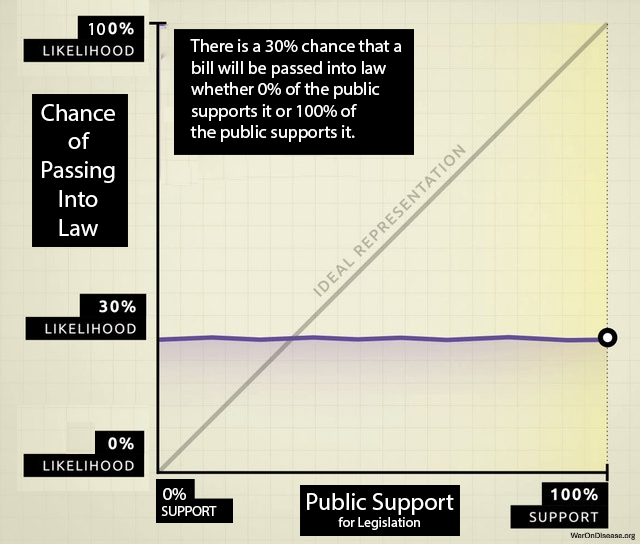
Empirical evidence confirms this pattern. Gilens and Page134 analyzed 1,779 policy decisions over two decades. Finding: “economic elites and organized groups representing business interests have substantial independent impacts on U.S. government policy, while mass-based interest groups and average citizens have little or no independent influence.” The correlation between average citizen preferences and policy outcomes was effectively zero. Whether 0% or 100% of citizens supported a policy, its probability of adoption remained unchanged at approximately 30%. By contrast, policies favored by economic elites were adopted at significantly higher rates. Figure 2 illustrates this disconnect.
1.2 Key Results
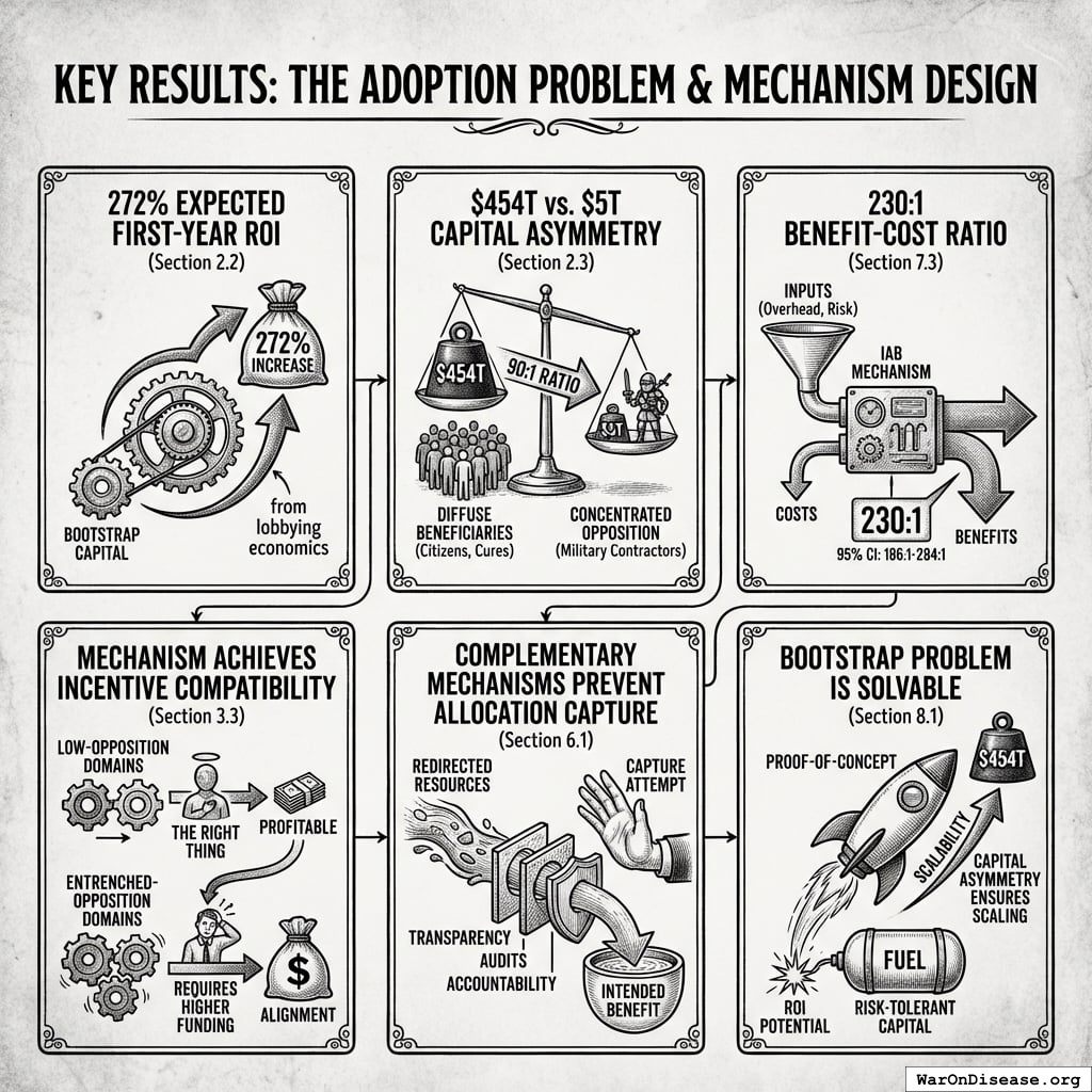
This paper demonstrates that the adoption problem (getting welfare-improving policies passed despite concentrated opposition) is solvable through mechanism design (designing rules so people’s selfish choices create good outcomes):
- 272% expected first-year ROI on bootstrap capital from lobbying economics (Section 2.2)
- $454T vs. $5T capital asymmetry ensures diffuse beneficiaries (citizens who’d benefit from cures) can outspend concentrated opposition (military contractors) by 90:1 (Section 2.3)
- 230:1 (95% CI: 186:1-284:1) benefit-cost ratio of the IAB mechanism itself, even accounting for overhead costs and failure risk (Section 7.3)
- Mechanism achieves incentive compatibility (when doing the right thing is also the profitable thing) with realistic parameters in low-opposition domains; requires higher funding in entrenched-opposition domains (Section 3.3)
- Complementary mechanisms prevent allocation capture once resources are redirected (Section 6.1)
- Bootstrap problem is solvable: ROI potential attracts risk-tolerant capital; capital asymmetry ensures scalability once proof-of-concept succeeds (Section 8.1)
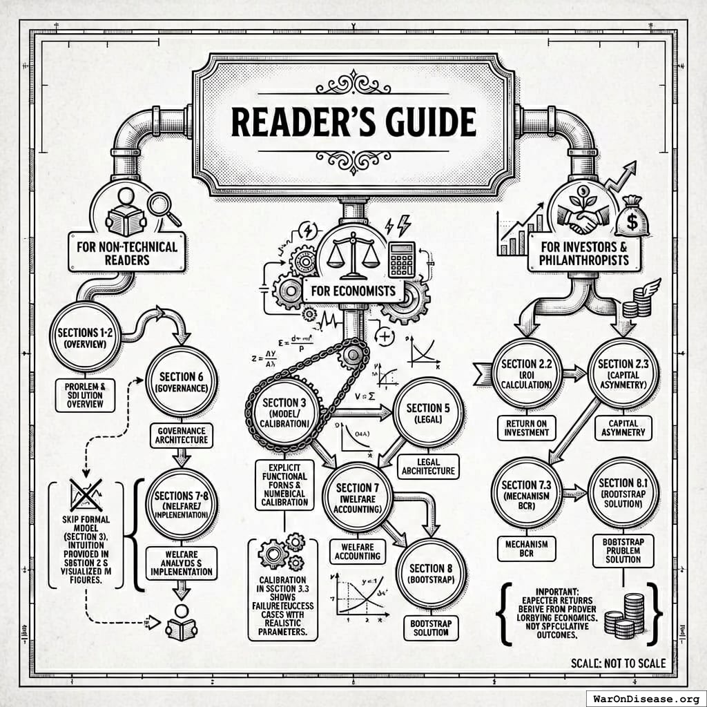
1.3 Reader’s Guide
Non-technical readers can skip Section 3 (formal model); the intuition is provided in Section 2. Economists should focus on Section 3 (explicit functional forms) and Section 7 (welfare accounting). Investors should focus on Section 2.2-2.3 (ROI and capital asymmetry) and Section 8 (bootstrap solution).
This paper introduces Incentive Alignment Bonds (IABs), a mechanism design approach to reversing this dynamic. Rather than attempting to change politicians’ preferences or relying on benevolent decision-makers, IABs restructure the incentive environment so that rational self-interest points toward welfare-improving policies.
1.4 Definition
An Incentive Alignment Bond is a financial instrument with three primitive properties:
- Investor alignment with public good production: Investors receive returns proportional to verified public-good funding flows achieved (e.g., treaty ratification, appropriations enacted). Returns are keyed to observable funding events, not downstream outcomes, avoiding complex attribution problems. If the policy succeeds, investors profit; if it fails, they do not. This creates a class of actors with concentrated financial interest in policy success.
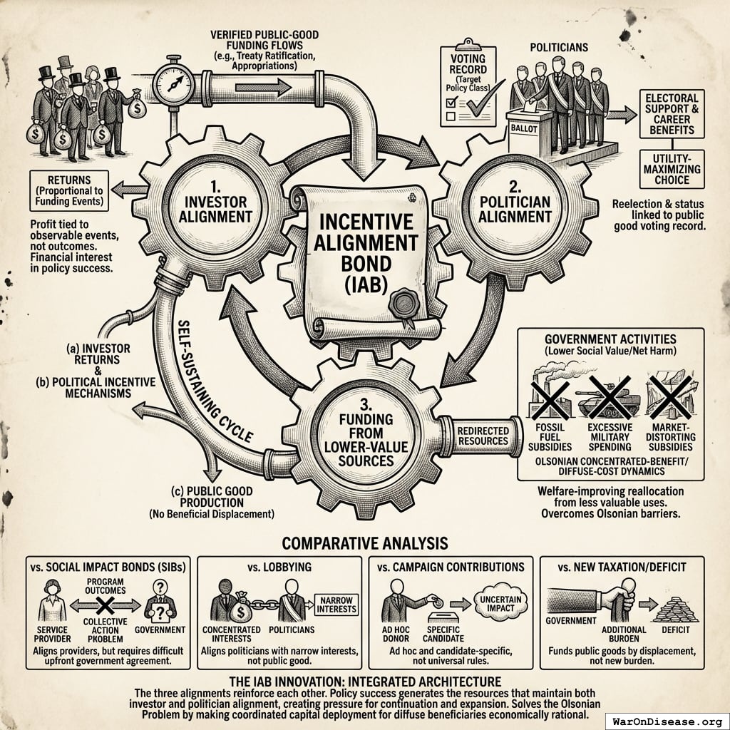
Politician alignment with public good production: Politicians receive electoral support and career benefits based on their voting record for the target policy class. Supporting the public good becomes the utility-maximizing choice, increasing reelection probability, post-office income, and status.
Funding from lower-value sources: The public good is funded by redirecting resources from government activities with lower social value than the target use. In the strongest case, these are programs that produce measurable net harm. More generally, they are programs that persist due to Olsonian concentrated-benefit/diffuse-cost dynamics rather than comparative merit. This constraint ensures IABs reallocate from less valuable to more valuable uses; they are welfare-improving in expectation under standard utilitarian social welfare assumptions.
The third property is crucial. Many government expenditures persist not because they produce social value, but because their beneficiaries are concentrated while their costs are diffuse. Military spending beyond deterrence requirements. Agricultural subsidies that distort markets. Fossil fuel subsidies that accelerate climate change. These programs survive political competition not on merit but on lobbying intensity. Concentrated interests (military contractors, incumbent industries) invest heavily in maintaining these programs, while diffuse beneficiaries face collective action problems. IABs redirect these resources to measurable public goods, making the reallocation welfare-improving even before accounting for the public good produced.
The key innovation is that all three alignments reinforce each other. A fraction of redirected funding flows perpetually to (a) investor returns and (b) political incentive mechanisms, while (c) the funding source ensures no beneficial programs are displaced. This makes the instrument self-sustaining: policy success generates the resources that maintain both investor and politician alignment, creating pressure for continuation and expansion.
Unlike Social Impact Bonds (which align service providers with program outcomes), IABs align the actors who control large-scale budget decisions, the politicians, with public-good production. Unlike lobbying (which aligns politicians with narrow interests), IABs align politicians with measurable, welfare-improving outcomes. Unlike campaign contributions (which are ad hoc and candidate-specific), IABs create universal, ex-ante rules tied to objective metrics. And unlike new taxation or deficit spending, IABs fund public goods by displacing harmful or wasteful expenditure.
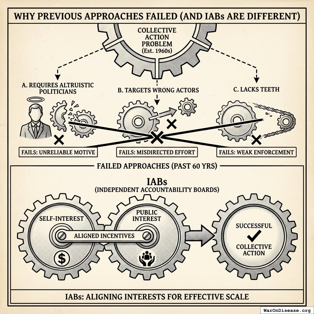
A natural objection: “How is this not just PACs + voter scorecards + SIBs?” The answer is that existing mechanisms fail to solve the Olsonian problem because they operate in isolation. PACs exist but remain dominated by concentrated interests due to the 90:1 capital asymmetry. Scorecards exist (League of Conservation Voters, NRA ratings) but lack teeth without accompanying financial incentives. SIBs exist but require government to agree upfront, which faces the same collective action problem IABs solve. IABs integrate all three components (investor capital, electoral accountability, post-office incentives) into a single instrument where each component’s effectiveness depends on the others, and where the funding mechanism creates permanent financial incentives for diffuse beneficiaries to overcome collective action barriers. The whole is greater than the sum of its parts because the integrated architecture makes coordinated capital deployment economically rational for millions of individual investors.
1.5 Why Reallocation, Not Addition
A natural question: why insist on redirecting resources from harmful programs rather than simply adding new spending on public goods? The answer: real resources (people, factories, scientists) are finite.
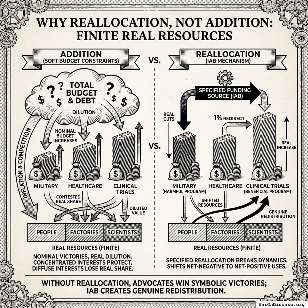
When advocates successfully lobby for increased spending on a beneficial program, the political response is rarely a corresponding reduction in harmful programs. Instead, governments usually:
- Expand the overall budget through deficit spending or monetary expansion
- Increase spending on politically powerful programs in parallel, to maintain coalition support
- Dilute the real value of new spending through inflation and competition for fixed resources
The result is that the beneficial program’s nominal budget increases while its real share of resources remains unchanged or even decreases. The concentrated beneficiaries of harmful programs lose nothing; the diffuse beneficiaries of the new program gain less than the headline figures suggest.
Consider the empirical pattern: between 2000 and 2024, U.S. federal spending on both military and healthcare increased much in nominal terms. Neither constituency “lost” to the other. Instead, total federal spending grew from $1.8 trillion to $6.1 trillion, while the national debt expanded from $5.6 trillion to $34 trillion. The real constraint, the finite pool of engineers, scientists, manufacturers, and productive capacity, was diluted across an ever-expanding set of nominal claims. Defense contractors retained their share of real resources; healthcare advocates won nominal victories that competed with inflation and expanding claims elsewhere in the budget.
This is not a failure of advocacy. It is the equilibrium outcome (stable result when everyone optimizes given current rules) of Olsonian dynamics operating under soft budget constraints (when governments can spend without immediate consequences; they just print money or charge it to the credit card of future generations). Concentrated interests protect their programs absolutely. Diffuse interests win nominal victories. The budget grows in nominal terms while each program’s claim on real resources remains contested.
The mechanism is straightforward: when Congress appropriates $10 billion for pragmatic clinical trials without specifying a funding source, the Treasury either borrows or the Federal Reserve accommodates. Total nominal spending increases.
But the supply of trained researchers, laboratory equipment, and institutional capacity does not increase proportionally. The new dollars compete with existing dollars, including those flowing to military, fossil fuel subsidies, and other Olsonian programs, for the same finite resources.
Inflation, both general and sector-specific, erodes the real purchasing power of the nominal increase.
IABs break this dynamic by specifying the funding source as part of the mechanism. The policy does not say “fund pragmatic clinical trials”; it says “redirect 1% of military spending to pragmatic clinical trials.” This forces a real reallocation:
- Military budgets face actual cuts in nominal and real terms
- Concentrated losers (military contractors) face real losses, which they will resist
- But the IAB political incentive layer ensures politicians who support the reallocation benefit more than those who resist
- The finite pool of resources shifts from net-negative to net-positive uses
The third primitive property, funding from harmful sources, is therefore not merely a normative preference or a political strategy. Under the soft budget constraint dynamics described above, it is enough to achieve real resource reallocation (likely needed in practice). Without specifying the funding source, advocates win symbolic victories while real resources continue flowing to Olsonian programs. With specified reallocation, the IAB creates genuine redistribution from net-negative to net-positive uses, constrained only by political will rather than by the illusion of unlimited budgetary capacity.
1.6 Political Change as an Asset Class
To understand why investors would fund the initial campaign to pass an IAB treaty, we must recognize political advocacy not as charity, but as a high-yield asset class. The Return on Investment (ROI) for corporate lobbying is historically orders of magnitude higher than traditional financial markets. The following illustrative estimates, drawn from existing studies, suggest order-of-magnitude returns:
- Defense: The top five military contractors spent $1.1 billion on lobbying over two decades while receiving $2.02 trillion in Pentagon contracts, an implied maximum ROI of approximately 181,000% assuming full attribution135.
- Fossil Fuels: The oil and gas industry spent $151 million lobbying in 2024 to protect $17 billion in subsidies, an implied maximum annual return of approximately 11,000% assuming full attribution136.
- Medical Research: Academic analysis finds that for specific disease groups, each $1,000 spent on lobbying is associated with $25,000 in additional NIH funding, an implied return of approximately 2,500%137.
These figures represent upper bounds assuming all contracts/subsidies are attributable to lobbying; causal attribution is complex and effects vary by context. Academic estimates of causal lobbying returns typically find 100-1000x ROI. Nevertheless, they suggest that political influence generates returns far exceeding traditional asset classes (compare to the S&P 500’s historical average of ~10%). Political change is currently accessible only to concentrated industries protecting the status quo. IABs securitize this opportunity, allowing investors to capture a fraction of the value generated by shifting government priorities toward public goods.
\[ E[R] = \frac{P(\text{success}) \times (\text{Redirected Flow} \times \text{Investor Share})}{\text{Campaign Cost}} \]
Illustrative calculation: If a campaign costs $1B and has a 20% chance of passing a treaty that redirects $27.2B/year (with 10% to investors), the expected annual value is:
\[ E[V] = 0.20 \times \$2.72\text{B} = \$544\text{M/year} \]
The expected first-year ROI on the $1B campaign is 54.4% (expected payout divided by campaign cost), with the revenue stream continuing in perpetuity. Upon treaty passage, the conditional ROI is 272%.
Sensitivity to parameter uncertainty:
| Parameter | Base Case | Effect on ROI |
|---|---|---|
| Success probability | 20% (illustrative) | Linear |
| Campaign cost | Inverse | |
| Investor share | 10% |
Linear |
| Treaty size | Linear |
Even under conservative assumptions (low success probability, upper CI bound on campaign cost, 10% investor share), expected ROI remains comparable to 10% stock market returns, with asymmetric upside. The mechanism is economically rational for risk-tolerant capital across a wide parameter range.
1.7 The Capital Asymmetry: Why IABs Can Outcompete Incumbent Lobbying
Here’s what almost everyone misses: the collective capital available to diffuse beneficiaries vastly exceeds the resources of concentrated interests. The problem is not lack of resources but lack of coordination.
Consider the global capital distribution:
- Concentrated interests (military contractors, fossil fuel companies, pharmaceutical incumbents): Combined market capitalization ~$5T1
- Diffuse beneficiaries (everyone who would benefit from cures, climate stability, pandemic prevention): Global household wealth ~$454T138
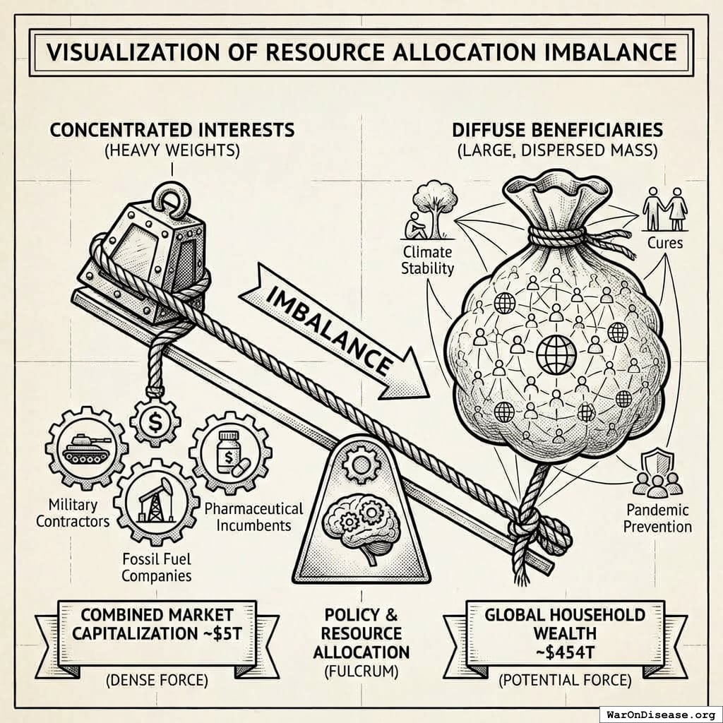
The 90:1 capital advantage cannot currently be deployed because diffuse beneficiaries face a collective action problem (hard for large groups to coordinate even when everyone would benefit): each individual’s stake is small, and coordination costs are prohibitive. A retiree who would gain 5 additional healthy years from accelerated medical research has enormous stake (~$500K in value of statistical life-years) but cannot coordinate with millions of other retirees to match pharmaceutical lobbying budgets.
IABs solve the coordination problem by securitizing political change (turning policy outcomes into tradable financial instruments, like turning mortgages into mortgage-backed securities). If IABs can be structured as tradable securities that any individual can purchase, they transform diffuse beneficiaries into the largest special interest group in history. The mechanism:
- Investment accessibility: Structure IABs as securities available to retail investors (similar to green bonds or social impact bonds)
- Returns exceed alternatives: Expected returns of 100-1000%+ (from lobbying ROI) dramatically exceed stock market returns of 10%
- Massive capital mobilization: Even 0.1% of global household wealth ($454T 0.1%) exceeds total annual global lobbying spending by 100×
- Self-interest alignment: Investors profit directly from policy success, creating concentrated financial incentives on the welfare-improving side
This reverses the Olsonian asymmetry. Defense contractors spend $100M+ annually lobbying because each firm captures concentrated benefits.
But the IAB mechanism allows millions of diffuse beneficiaries to collectively deploy billions while each capturing a proportional return.
The concentrated opposition ($100M-$1B annually) becomes outmatched by newly-coordinated diffuse support ($10B-$100B+ available capital).
We’re not inventing lobbying. Defense contractors proved it works decades ago. We’re just making it available to everyone whose lives depend on cures instead of bombs. Turns out there are more of us, and we’re much richer. The political change ROI (100-10,000x) that currently accrues only to concentrated industries becomes accessible to everyone who benefits from public goods.
1.8 Quantifying Net Societal Value of Funding Sources
The third primitive property requires identifying government expenditures with lower marginal social value than the proposed alternative. This is an empirical question that can be addressed using standard welfare economics:
\[ NSV_i = B_i - C_i \tag{1}\]
where \(NSV_i\) is net societal value of program \(i\), \(B_i\) is measurable social benefits (including economic multiplier effects), and \(C_i\) is total costs (including both direct expenditure and opportunity costs of foregone alternatives).
A program is an appropriate IAB funding source if:
\[ NSV_{source} < NSV_{target} \tag{2}\]
That is, if the marginal social value of the source program is lower than that of the target program. In the strongest case, \(NSV_{source} \leq 0\); the program produces net harm. But reallocation is justified even when both programs have positive value, as long as the target exceeds the source.
This comparative criterion implies a natural ranking of government expenditures by marginal social value. IABs should draw from the lowest-ranked programs first, those that persist mainly due to Olsonian dynamics rather than merit. This avoids the objection that “military isn’t ALL bad”; the claim is not that military spending is worthless, but that its marginal value is lower than medical research, and that it persists at current levels due to lobbying intensity rather than comparative social value.
Military spending provides a concrete example. The economic multiplier for military spending is around 0.6, compared to 1.5–3.0 for infrastructure, education, and medical research. This means each dollar of military spending generates $0.60 in economic activity, while each dollar of medical research investment generates $2.00–3.00. The opportunity cost alone, before considering direct harms, makes military spending beyond minimum deterrence requirements a net social loss.
More comprehensive analysis includes:
| Cost Category | Annual Value | Source |
|---|---|---|
| Direct military expenditure | ||
| Lost GDP from multiplier differential | ||
| Infrastructure destruction (active conflicts) | World Bank | |
| Human casualties (VSL method) | EPA VSL × conflict deaths | |
| Trade disruption | World Bank trade flow analysis | |
| Veteran healthcare (ongoing) | ||
| Environmental damage | ||
| Total societal cost | $11.4T (95% CI: $9.01T-$14.1T) | Sum of above |
A large literature suggests the net societal value of military spending beyond minimum deterrence is strongly negative: $2.72T in direct expenditure produces $11.4T (95% CI: $9.01T-$14.1T) in societal costs (see Table 1 for illustrative order-of-magnitude estimates). If these estimates are roughly correct, redirecting even 1% to pragmatic clinical trials, which has positive externalities and high multipliers, would be welfare-improving on net.
Similar analysis applies to other Olsonian programs:
- Fossil fuel subsidies ($7T globally, IMF 2023): Accelerate climate change, distort energy markets, produce negative externalities exceeding subsidy value
- Agricultural subsidies in developed nations: Distort global food markets, harm developing-country farmers, produce environmental damage from monoculture incentives
- Regulatory capture programs: Expenditures that exist to protect incumbent firms from competition rather than serve public interest
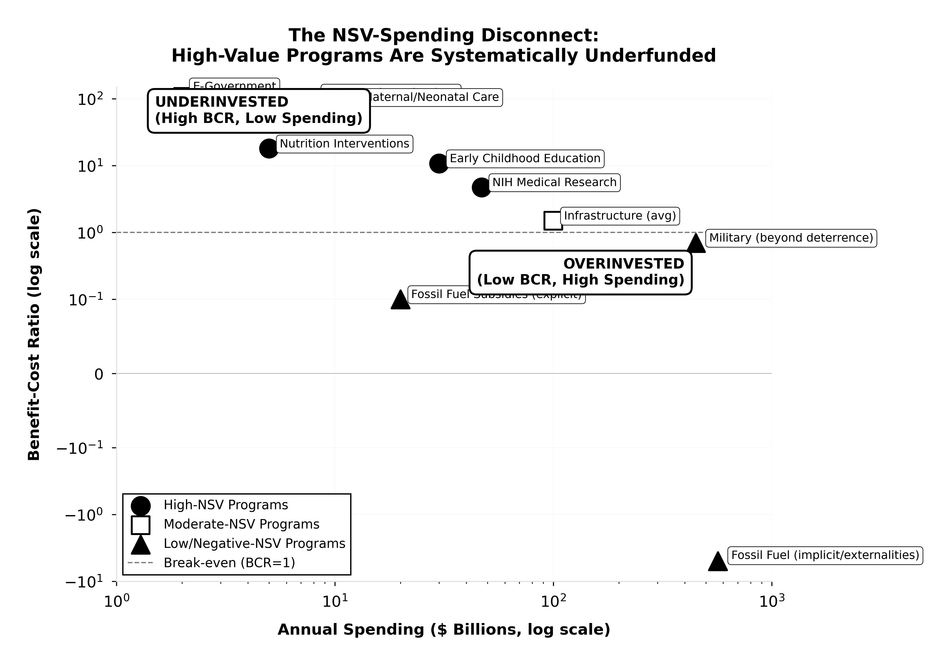
Table 2 presents a comprehensive ranking combining Copenhagen Consensus data with other authoritative sources. The pattern is stark: programs with BCRs exceeding 100:1 receive single-digit billions in annual spending, while programs with negative NSV receive hundreds of billions. Spending correlates with lobbying intensity, not social value. This systematic misallocation is the empirical foundation for the IAB mechanism.
| Program / Category | BCR | Annual Spending | Est. NSV (per $1) | Source |
|---|---|---|---|---|
| HIGH-NSV PROGRAMS (IAB TARGETS) | ||||
| Pragmatic Clinical Trials | 637:1 – 11,540:1 | ~$60B | +$636 – $11,539 | 139;140 |
| Childhood Vaccinations (Global) | 101:1 | ~$8B | +$100 | Copenhagen Consensus 2023132 |
| E-Government Procurement | 125:1 | ~$2B | +$124 | Copenhagen Consensus 2023132 |
| Maternal/Neonatal Care | 87:1 | ~$12B | +$86 | Copenhagen Consensus 2023132 |
| Nutrition Interventions | 18:1 | ~$5B | +$17 | Copenhagen Consensus 2023132 |
| Medical Research (NIH) | 2.56:1 – 4.75:1 | $47B | +$1.56 – $3.75 | United for Medical Research141 |
| Early Childhood Education | 2.5:1 – 10.8:1 | ~$30B | +$1.50 – $9.80 | 142,143 |
| MODERATE-NSV PROGRAMS | ||||
| Infrastructure (High-Quality) | 1.5:1 – 2.5:1 | Varies | +$0.50 – $1.50 | 144; highly project-dependent |
| LOW/NEGATIVE-NSV PROGRAMS (IAB SOURCES) | ||||
| Military (Beyond Deterrence) | ~0.7:1 | $450B+ (US) | -$0.30 | 145; fiscal only, excludes conflict costs |
| Fossil Fuel Subsidies (Explicit) | <0 | $20B (US) | -$1 to -$5 | 111 |
| Fossil Fuel (Implicit/Externalities) | -5:1 | $568B (US) | -$5 | 146, PNAS 2021 externality analysis |
The empirical criterion is straightforward: if a program’s beneficiaries are concentrated, its costs are diffuse, and rigorous cost-benefit analysis shows \(NSV_{source} < NSV_{target}\), reallocation is welfare-improving. In the clearest cases, where \(NSV_{source} \leq 0\), the source program is actively harmful and reallocation is unambiguously beneficial. But even programs with modestly positive NSV are appropriate sources if the target has much higher value. The IAB mechanism does not require moral judgment about the source program, only comparative measurement.
Under rational resource allocation, we would expect high-BCR programs to receive high spending (upper-right quadrant) and low-BCR programs to receive low spending (lower-left quadrant). Instead, we observe the opposite: programs with BCRs exceeding 100:1 are clustered in the “UNDERINVESTED” region, while programs with BCRs below 1:1 (or negative) are in the “OVERINVESTED” region.
This systematic misallocation is the empirical foundation for Incentive Alignment Bonds: spending correlates with lobbying intensity, not social value.
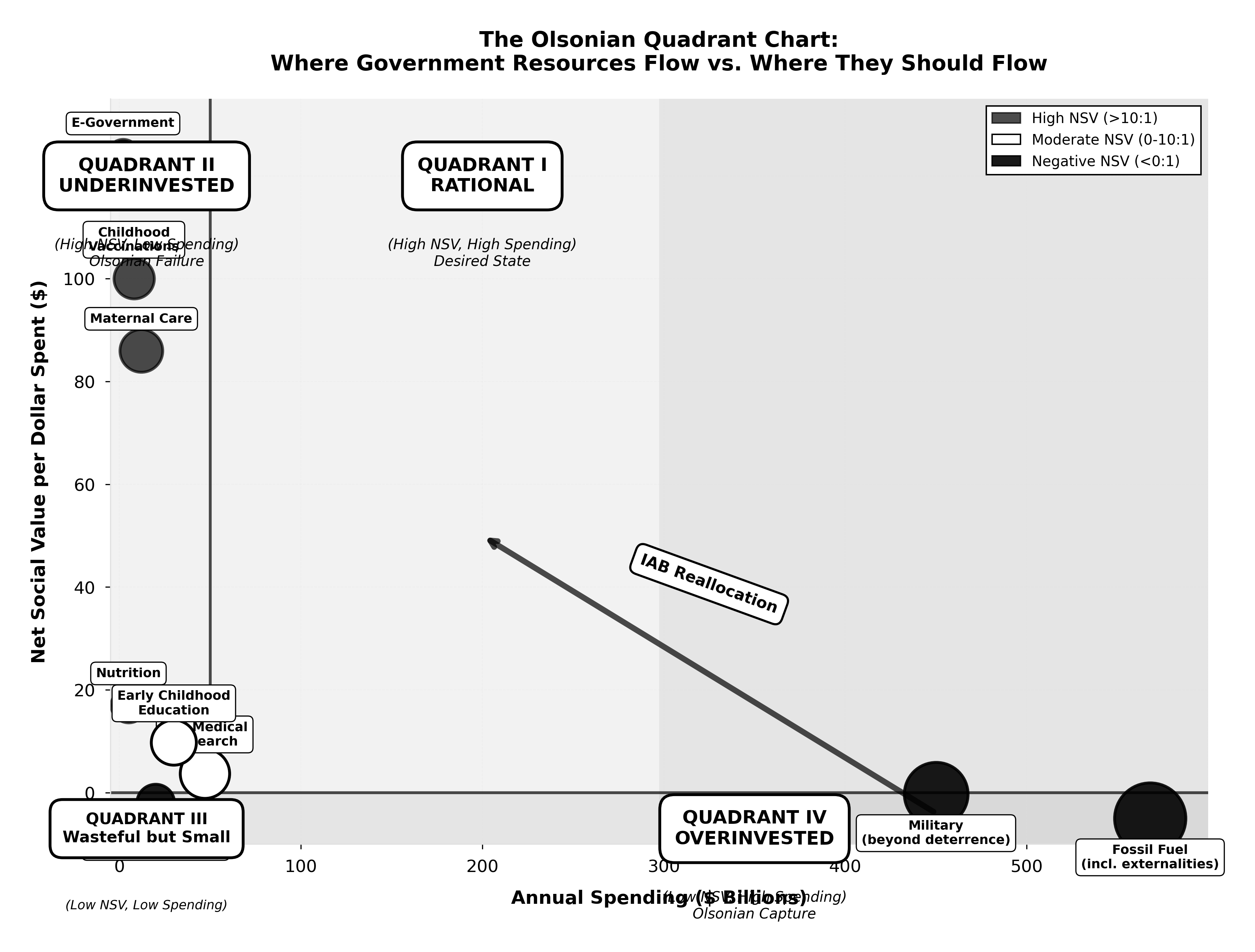
Interpretation:
- Quadrant I (Rational): Programs with high NSV receiving high spending: the desired equilibrium
- Quadrant II (Underinvested): High-NSV programs receiving low spending: Olsonian failure where diffuse benefits cannot coordinate
- Quadrant III (Wasteful but Small): Low-NSV programs with low spending: wasteful but limited damage
- Quadrant IV (Overinvested): Low-NSV programs receiving high spending: Olsonian capture where concentrated interests dominate
The IAB Mechanism: Redirects resources from Quadrant IV → Quadrant I by making politician support for high-NSV programs individually rational through score-dependent electoral and career benefits.
Figure 3 visualizes this systematic misallocation as a scatter plot, while Figure 4 categorizes programs into four quadrants based on their NSV and funding levels. These visualizations make clear that under rational allocation, high-BCR programs receive high funding (upper-right quadrant). Instead, we observe the opposite: high-BCR programs cluster in the “UNDERINVESTED” region while low/negative-BCR programs are “OVERINVESTED.”
1.9 Relation to Existing Literature
This paper combines three literatures. First, mechanism design theory147–149 provides tools for designing institutions when agents have private information and act strategically. While mechanism design has transformed market institutions, from spectrum auctions150 to kidney exchanges151, its application to political institutions is limited. We extend this framework to political incentives, treating politicians as strategic agents whose actions (votes) are observable but whose preferences may diverge from social welfare.

Second, public choice theory133,152 models politicians as utility maximizers rather than benevolent planners. Olson’s analysis of concentrated versus diffuse interests explains persistent policy failures but offers limited remedies. We turn Olson’s insight into a mechanism: if concentrated benefits cause politicians to favor narrow interests, then concentrating benefits on the welfare-improving side can reverse the dynamic.
Third, campaign finance research153–155 and political agency models156 document how electoral incentives and career concerns shape politician behavior. We synthesize these findings into a mechanism that systematically exploits these channels for public goods.
Relative to Social Impact Bonds157,158, IABs target a different agent (politicians vs. service providers) at a different level (policy adoption vs. program delivery). Relative to lobbying and campaign contributions, IABs create universal, ex-ante, public rules tied to verifiable outcomes rather than ad hoc relationships. Relative to pure voting reform proposals, IABs work within existing institutional constraints.
1.10 Contribution
This paper makes four contributions:
- Mechanism Design for Governance: We apply the formal tools of mechanism design theory, developed for auctions, matching markets, and resource allocation, to the problem of political incentives. While mechanism design has transformed economic institutions from spectrum auctions to kidney exchanges, its application to democratic governance is underdeveloped.
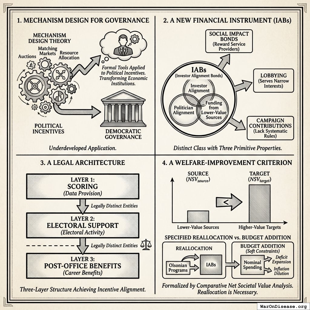
A New Financial Instrument: We define IABs as a distinct class of financial instrument with three primitive properties: investor alignment, politician alignment, and funding from lower-value sources. This distinguishes IABs from Social Impact Bonds (which reward service providers, not politicians), lobbying (which serves narrow interests), and campaign contributions (which lack systematic, ex-ante, universal rules tied to measurable outcomes).
A Legal Architecture: We specify a three-layer structure (scoring, electoral support, post-office benefits) that achieves incentive alignment without violating anti-bribery statutes. The legal innovation is separating data provision from electoral activity from career benefits, with each layer operated by legally distinct entities.
A Welfare-Improvement Criterion: We formalize how to identify appropriate IAB funding sources using comparative net societal value analysis (\(NSV_{source} < NSV_{target}\)) and show why specified reallocation, rather than budget addition, is enough (needed) to achieve real resource shifts. Under soft budget constraints, nominal spending increases are diluted by deficit expansion and inflation while Olsonian programs retain their share of real resources. This comparative criterion implies a natural ranking of expenditures; IABs draw from the lowest-ranked programs first, ensuring reallocation is welfare-improving under standard utilitarian assumptions.
1.11 Roadmap
Section 2 reviews why previous approaches failed. Section 3 presents the formal model. Section 4 details the three-layer architecture and its legal basis. Section 5 analyzes failure modes. Section 6 discusses the broader governance stack. Section 7 extends the mechanism to climate, nuclear risk, and pandemic preparedness. The Conclusion summarizes contributions and open questions.

2 Why Previous Approaches Failed
2.1 Mechanism Design Theory
The Sveriges Riksbank Prize in Economic Sciences 2007 was awarded to Leonid Hurwicz, Eric Maskin, and Roger Myerson “for having laid the foundations of mechanism design theory”159. Mechanism design addresses a fundamental problem: how do you get selfish people to do the right thing without forcing them?
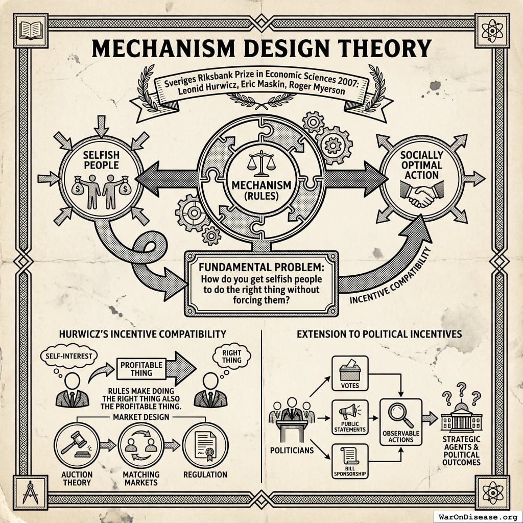
Hurwicz147 introduced the concept of incentive compatibility: a mechanism is incentive-compatible if the socially optimal action is in each agent’s self-interest. The rules make doing the right thing also the profitable thing.
These concepts have transformed market design: auction theory150, matching markets151, and regulation160. This paper extends mechanism design to political incentives, treating politicians as strategic agents whose actions (votes, public statements, bill sponsorship) are observable.
2.2 Public Choice Theory
Public choice theory applies economic methods to political behavior. Buchanan and Tullock152 model politicians and voters as rational utility maximizers, not benevolent social planners. Olson133 shows that collective action for public goods is systematically undersupplied because:
- Free-rider problem: Large groups cannot exclude non-contributors from benefits
- Asymmetric stakes: Per-member stakes are higher in small groups
- Organization costs: Smaller groups face lower coordination costs
The result is that “concentrated minor interests will be overrepresented and diffuse majority interests trumped”133. Empirical support includes Lohmann’s observation that U.S. sugar import quotas generated 2,261 jobs while reducing overall welfare by $1.162 billion, an implicit cost per job exceeding $500,000161. The government could have paid each sugar worker half a million dollars to not grow sugar. This would have saved money. Nobody did this. Sugar growers have lobbyists. Consumers don’t.
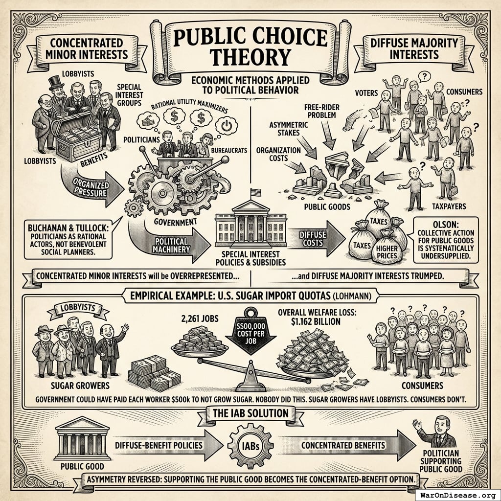
IABs address this directly: by concentrating benefits on politicians who support diffuse-benefit policies, the asymmetry is reversed. Supporting the public good becomes the concentrated-benefit option.
2.4 Campaign Finance and Political Behavior
Empirical research on campaign finance provides the evidentiary foundation for the electoral layer of IABs.
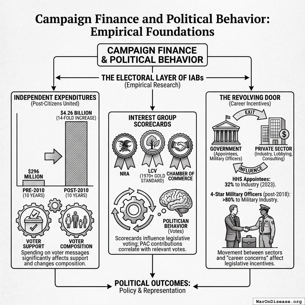
Independent expenditures affect elections. Following Citizens United v. FEC (2010), independent expenditures increased dramatically. In the decade prior to the decision, outside groups spent $296 million total on independent expenditures; in the decade after, they spent $4.26 billion, a 14-fold increase164. Research using transaction-level disbursement data finds that “spending on messages to voters has a statistically significant effect on voter support for candidates” and is “especially effective in changing the composition of voters”153.
Interest group scorecards influence behavior. Organizations like the National Rifle Association (NRA), League of Conservation Voters (LCV), and Chamber of Commerce publish voting scorecards that affect politician behavior. The LCV has published its National Environmental Scorecard since 1970, and it has “become the gold standard of congressional vote scoring on environmental issues”165. Research confirms that PAC contributions correlate with votes on relevant issues, though causality is debated154,155.
The revolving door affects politician incentives. Research documents significant movement between government and private sector. A 2023 study found that 32% of HHS appointees exited to industry employment166. Among four-star military officers who retired after June 2018, over 80% went to work for the military industry as board members, advisors, executives, consultants, or lobbyists167. Shepherd and You156 find evidence that “career concerns” about post-office employment influence legislative behavior.
2.5 Credit Rating Agencies as Governance Mechanisms
Credit rating agencies (CRAs) provide a precedent for private organizations influencing sovereign policy through reputational mechanisms. Moody’s, S&P, and Fitch assign sovereign credit ratings that directly affect borrowing costs. Barta168 describes CRAs as “unelected, unappointed, unaccountable profit-seeking institutions” whose power rivals the IMF or World Bank. Downgrades can trigger crises: Greece, Ireland, and Portugal all experienced accelerated debt crises following CRA downgrades to “junk” status169.
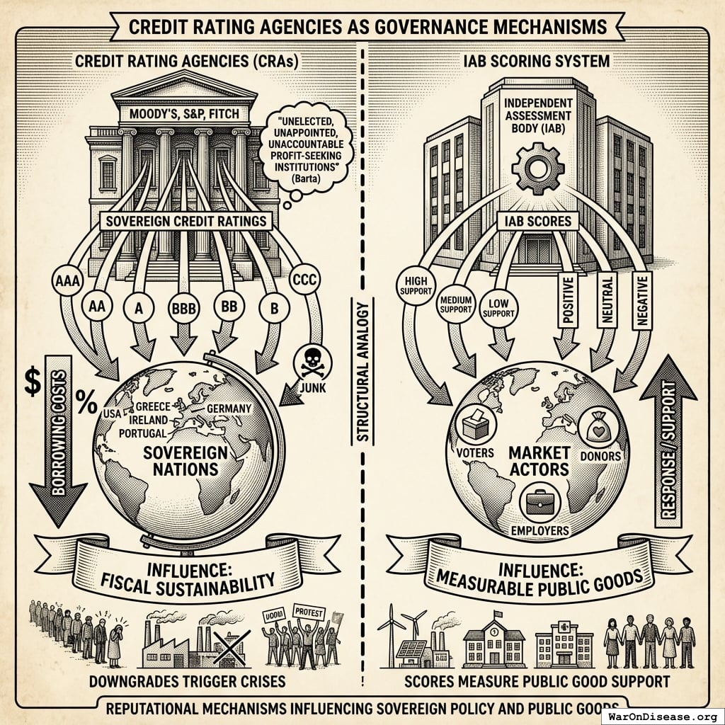
The IAB scoring system is structurally analogous to credit ratings: an independent body publishes scores based on objective criteria, and market actors (voters, donors, employers) respond to those scores. The difference is the metric: instead of fiscal sustainability, IABs measure support for measurable public goods.
3 The Math: Proving It Works
For Non-Technical Readers: You can skip this section. In plain English: We create a “Public Good Score” for each politician based on their voting record. Politicians with higher scores get (1) campaign support from independent political groups, (2) better post-office job opportunities, and (3) higher public status. When these benefits exceed the costs (losing military contractor donations), supporting public goods becomes the rational choice. Skip to Section 4 for practical implementation or Section 6 for governance architecture.
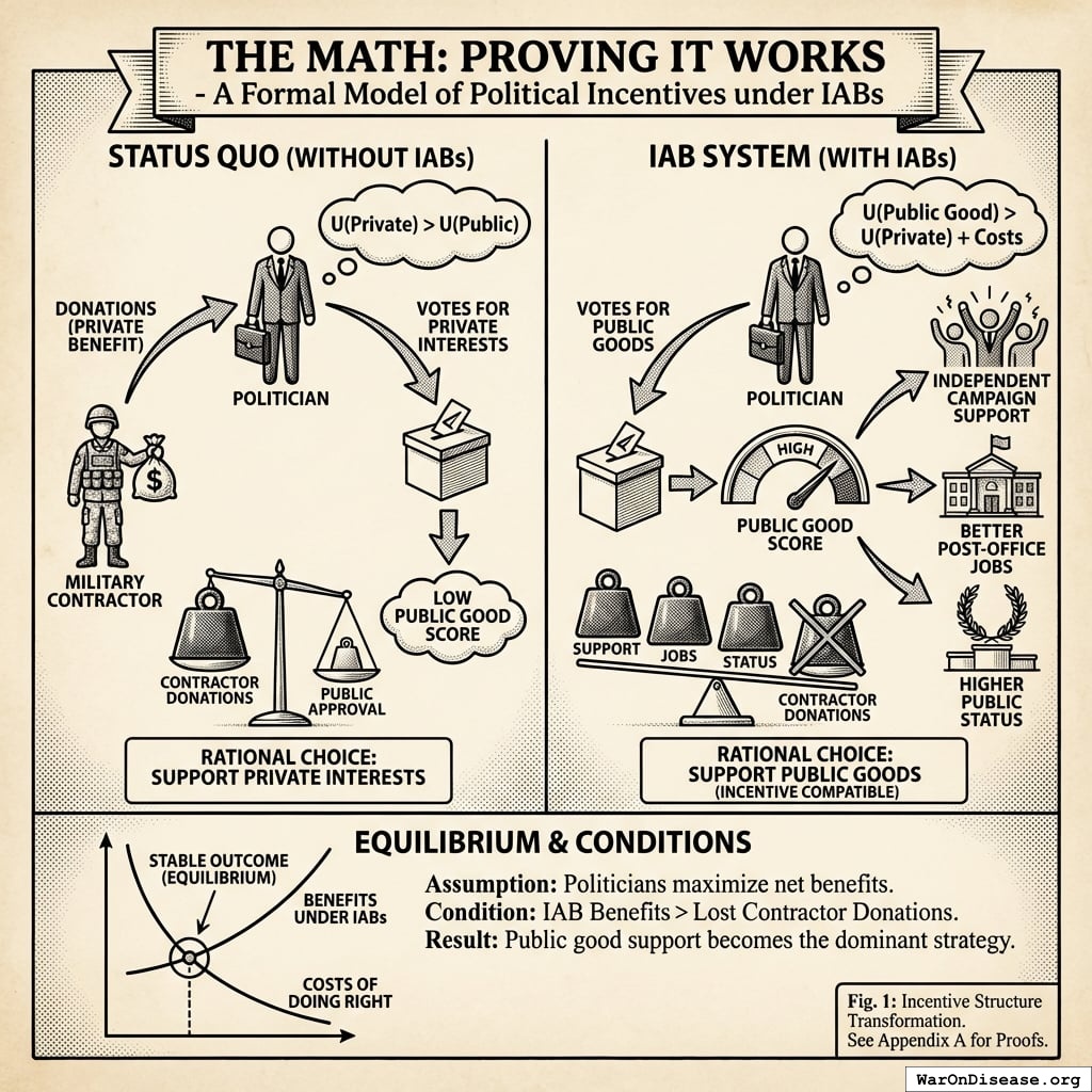
This section presents a formal model of political incentives under IABs. We state explicit assumptions, derive conditions for incentive compatibility (when doing the right thing is also the profitable thing), and characterize equilibria (stable outcomes). Appendix A provides detailed proofs.
3.1 Assumptions
We maintain the following assumptions throughout:
A1 (Rational Politicians). Each politician \(i \in \{1, \ldots, N\}\) is a rational agent maximizing expected utility \(U_i\) over career outcomes, including reelection, post-office income, and legacy.
A2 (Observable Votes). Voting records on policy class \(\mathcal{P}\) are publicly observable and verifiable. The scoring function \(f: \text{VoteRecord} \to \mathbb{R}\) is common knowledge.
A3 (Credible Commitment). The IAB mechanism can credibly commit to score-dependent payoffs: independent expenditure rules \(I_i(\theta_i)\) and post-office eligibility criteria \(\tau(\theta_i)\) are announced ex ante and cannot be renegotiated ex post.
A4 (Funded Mechanism). The IAB is sufficiently capitalized that the payoff differentials \(\Delta P_i\), \(\Delta Y_i\) induced by score changes are non-negligible relative to concentrated opposition costs \(c_i\).
A5 (Single Policy Dimension). Politicians face a binary choice \(a_i \in \{0,1\}\) on the target policy class. Extensions to multiple dimensions are discussed in Section 6.
3.2 The Politician’s Utility Function
We model a politician \(i\) as a rational agent maximizing a utility function:
\[ U_i = \alpha_i \cdot P_i(\text{reelection}) + \beta_i \cdot E_i[\text{PostOfficeIncome}] + \gamma_i \cdot S_i(\text{Legacy}) \tag{3}\]
where:
- \(P_i(\text{reelection})\) is the probability of winning the next election
- \(E_i[\text{PostOfficeIncome}]\) is expected lifetime earnings after leaving office
- \(S_i(\text{Legacy})\) is a status/legacy function (books, buildings named, Wikipedia length)
- \(\alpha_i, \beta_i, \gamma_i > 0\) are weights varying by politician but assumed positive
This formulation is consistent with public choice theory’s treatment of politicians as utility maximizers152 and with empirical research on career concerns156.
3.3 The Utility Function Transformation
The key mechanism design insight is that IABs transform the politician’s utility function by introducing a dependency on net societal value (NSV) rankings through an intermediate score variable.
Pre-IAB utility function: Let \(R\) denote the ranking of programs by NSV (as produced by Copenhagen Consensus, GiveWell, etc.). In the status quo:
\[ U_i^{\text{pre-IAB}} = \alpha_i \cdot P_i + \beta_i \cdot Y_i + \gamma_i \cdot S_i \tag{4}\]
Critically, the ranking \(R\) appears nowhere in this function. Each component is driven by lobbying intensity and concentrated interests, not social value:
- \(P_i = P_i^0 + f(\text{campaign contributions}) + g(\text{attack ads avoided})\)
- \(Y_i = h(\text{revolving door relationships})\)
- \(S_i = s(\text{partisan loyalty}, \text{donor satisfaction})\)
Post-IAB utility function: The IAB mechanism introduces a Public Good Score \(\theta_i = f(R, \text{VoteRecord}_i)\) that translates the NSV ranking into politician-specific incentives. Each utility component becomes score-dependent:
\[ U_i^{\text{post-IAB}} = \alpha_i \cdot P_i(\theta_i) + \beta_i \cdot Y_i(\theta_i) + \gamma_i \cdot S_i(\theta_i) \tag{5}\]
Now the ranking \(R\) is operative through \(\theta_i\). Politicians who vote to reallocate resources from low-NSV to high-NSV programs see their scores rise, which increases their reelection probability, post-office income prospects, and legacy value.
Explicit functional forms: The post-IAB components are specified as:
Reelection probability:
\[ P_i(\theta_i) = P_i^0 + \delta \cdot (\theta_i - \bar{\theta}) + \epsilon_i \cdot I_i(\theta_i) \tag{6}\]
where \(P_i^0\) is baseline reelection probability, \(\bar{\theta}\) is the median score, \(\delta > 0\) captures the direct electoral effect of scorecard visibility, and \(I_i(\theta_i)\) is the independent expenditure function (a step function with discrete rewards):
\[ I_i(\theta_i) = \begin{cases} +M & \text{if } \theta_i \geq \theta^{high} \\ 0 & \text{if } \theta^{med} \leq \theta_i < \theta^{high} \\ -M & \text{if } \theta_i < \theta^{med} \end{cases} \tag{7}\]
Post-office income:
\[ Y_i(\theta_i) = Y(\tau(\theta_i)) \tag{8}\]
where \(\tau: \mathbb{R} \to \{1, 2, 3\}\) maps scores to income tiers:
\[ \tau(\theta_i) = \begin{cases} 1 & \text{if } \theta_i \geq 75 \quad (\text{Tier 1: \$500K+ annually}) \\ 2 & \text{if } 60 \leq \theta_i < 75 \quad (\text{Tier 2: \$200-400K annually}) \\ 3 & \text{if } \theta_i < 60 \quad (\text{Tier 3: \$150-300K annually}) \end{cases} \tag{9}\]
Legacy/status:
\[ S_i(\theta_i) = S_0 + \lambda \cdot \theta_i \tag{10}\]
where \(S_0\) is baseline status and \(\lambda > 0\) captures the marginal status gain from higher scores (measured by metrics such as Wikipedia article length, think tank fellowships, speaking invitations, historical assessments).
Generated: /home/runner/work/disease-eradication-plan/disease-eradication-plan/_build_temp/iab/knowledge/figures/utility-function-pre-iab.pngBefore IABs: Politicians maximize utility based on lobbying intensity. The NSV ranking exists but doesn’t affect their utility function, so they have no incentive to support high-NSV programs.
Generated: /home/runner/work/disease-eradication-plan/disease-eradication-plan/_build_temp/iab/knowledge/figures/utility-function-post-iab.pngAfter IABs: The same utility function becomes score-dependent: each component (electoral, career, legacy) now depends on the politician’s score, which is determined by their voting record on NSV-ranked programs. Supporting high-NSV programs becomes the rational, self-interested choice.
The transformation does not change what politicians optimize; it changes what optimizing points at. Same selfish utility maximization, radically different equilibrium outcome. This is the core mechanism design contribution: we align private incentives with public welfare not by appealing to altruism, but by redirecting self-interest. The diagrams above illustrate this transformation (compare Figure 5 with Figure 6).
3.4 Numerical Calibration and Parameter Ranges
To evaluate whether Equation 11 (the incentive compatibility condition) can realistically be satisfied, we provide illustrative calibrations based on campaign finance research and career trajectories.
Base case parameters:
| Politician Type | \(\alpha_i\) (Electoral Weight) | \(\beta_i\) (Career Weight) | \(\gamma_i\) (Legacy Weight) | \(P_i^0\) (Baseline Prob.) |
|---|---|---|---|---|
| Marginal seat | 0.6 | 0.3 | 0.1 | 0.50 |
| Safe seat | 0.2 | 0.5 | 0.3 | 0.85 |
| Termed out | 0.0 | 0.7 | 0.3 | N/A |
IAB mechanism parameters (illustrative):
- Score threshold for high tier: \(\theta^{high} = 80\), \(\theta^{med} = 60\)
- Independent expenditure support: \(M = \$5\text{M to }\$20\text{M}\) (competitive race)
- Electoral impact: \(\delta = 0.02\) to \(0.05\) (2-5 percentage point swing from scorecard visibility)
- Post-office income differential: \(\Delta Y = \$200\text{K to }\$350\text{K annually}\) (present value $3M-$5M over 15-year career)
- Legacy multiplier: \(\lambda = 0.1\) (1 SD score increase → 10% increase in Wikipedia length, fellowships, etc.)
Concentrated opposition cost:
- Moderate opposition: \(c_i = \$2\text{M to }\$5\text{M}\) (attack ads, lost contributions, primary challenge risk)
- Strong opposition: \(c_i = \$10\text{M to }\$20\text{M}\) (defense/fossil fuel reallocation)
Incentive compatibility calculation (marginal seat politician):
Suppose a marginal-seat Senator (50% baseline reelection, \(\alpha_i = 0.6\), \(\beta_i = 0.3\), \(\gamma_i = 0.1\)) votes for a 1% military reallocation treaty:
\[ \Delta P_i = \delta \cdot \Delta\theta + \epsilon_i \cdot M = (0.03)(20) + (0.08 \text{ pp}/\$\text{M})(\$10\text{M}) = 0.6\text{ pp} + 0.8\text{ pp} = 1.4\text{ pp} \]
Note: εi is calibrated in percentage points per $1M, so εi·M yields percentage points.
\[ \Delta Y_i = \$300\text{K annually} \times \frac{1 - (1.05)^{-15}}{0.05} \approx \$300\text{K} \times 10.38 \approx \$3.11\text{M PV} \]
\[ \Delta S_i = \lambda \cdot \Delta\theta = 0.1 \times 20 = 2.0 \]
Utility gain (converting all terms to dollar-equivalents, with reelection probability valued at $50M lifetime Senate seat value and status units at $10M each):
\[ \alpha_i \Delta P_i + \beta_i \Delta Y_i + \gamma_i \Delta S_i \approx 0.6(\$50\text{M} \times 0.014) + 0.3(\$3.11\text{M}) + 0.1(\$10\text{M} \times 2.0) \]
\[ \approx \$0.42\text{M} + \$0.93\text{M} + \$2\text{M} \approx \$3.35\text{M} \]
If concentrated opposition cost is \(c_i = \$5\text{M}\) (attack ads, lost defense PAC contributions), then:
\[ \Delta U_i = \$1.35\text{M} - \$5\text{M} = -\$3.65\text{M} < 0 \]
Mechanism fails with current calibration. To achieve incentive compatibility, IABs must increase either:
- Independent expenditure support (\(M\)) from $10M to $20M+
- Post-office income differential (\(\Delta Y\)) via additional tier benefits
- Electoral impact (\(\delta\)) through more aggressive scorecard visibility campaigns
Revised calibration (mechanism succeeds):
If \(M = \$20\text{M}\) and \(\delta = 0.05\):
\[ \Delta P_i = 0.05(20) + 0.08(\$20\text{M}) = 1.0 + 1.6 = 2.6\% \]
\[ \Delta U_i = 0.6(0.026)(\text{value of 2.6pp reelection}) + 0.3(\$4.5\text{M}) + 0.1(2.0) \]
Translating reelection probability to dollars (value of Senate seat ≈ $50M lifetime value):
\[ \Delta U_i \approx 0.6(0.026 \times \$50\text{M}) + \$1.35\text{M} + 0.2 \approx \$0.78\text{M} + \$1.35\text{M} = \$2.13\text{M} \]
Still insufficient if \(c_i = \$5\text{M}\). But if concentrated opposition is only \(c_i = \$2\text{M}\) (lower-opposition domain like pandemic preparedness), mechanism succeeds:
\[ \Delta U_i = \$2.13\text{M} - \$2\text{M} = \$0.13\text{M} > 0 \quad \checkmark \]
The calibration shows:
- Pandemic preparedness (\(c_i = \$1\text{M-}\$3\text{M}\)) is more tractable than defense reallocation (\(c_i = \$10\text{M-}\$20\text{M}\))
- Safe-seat politicians need larger \(\beta_i\) (career) and \(\gamma_i\) (legacy) incentives since \(\alpha_i\) (electoral) is small
- Termed-out politicians are most cost-effective: \(\alpha_i = 0\) but \(\beta_i = 0.7\) means post-office incentives dominate
- High-opposition domains require $20M+ per pivotal vote; low-opposition domains require $5M-$10M
Equation 16 is achievable with realistic parameter values in carefully-selected domains.
3.5 The Policy Choice
Consider a binary policy choice \(a_i \in \{0, 1\}\) where:
- \(a_i = 1\): Support a policy that funds public good \(G\)
- \(a_i = 0\): Oppose or abstain
Let \(W(G)\) denote the social welfare gain from \(G\). By assumption, \(W(G) > 0\); the policy is welfare-improving. The question is whether \(a_i = 1\) is incentive-compatible.
3.6 The Pre-IAB Equilibrium
Without IABs, the politician faces:
Benefits of \(a_i = 1\):
- Diffuse voter approval (small per-voter benefit, hard to attribute)
- Abstract “doing the right thing” utility (assumed small)
Costs of \(a_i = 1\):
- Concentrated opposition from losers (military contractors, pharmaceutical incumbents)
- Attack ads: “Senator voted to WEAKEN AMERICA”
- Loss of campaign contributions from concentrated interests
Formally:
\[ \Delta U_i^{\text{pre-IAB}}(a_i = 1) = \epsilon - c_i \tag{11}\]
where \(\epsilon\) is the small diffuse benefit and \(c_i > 0\) is the net concentrated cost from losing incumbents’ support (campaign contributions foregone, attack ads received, post-office opportunities closed). Since \(c_i > \epsilon\) for most policies with diffuse benefits, the equilibrium is \(a_i^* = 0\). This is Olson’s result in formal terms.
3.7 The IAB Mechanism
The IAB mechanism introduces a Public Good Score \(\theta_i\) for each politician, where:
\[ \theta_i = f(\text{VoteRecord}_i) \tag{12}\]
The score is based purely on voting record on policy class \(\mathcal{P}\) (policies meeting specified criteria for the target public good). This is a design choice with important implications:
- Measurability: Voting records are public, verifiable, and effectively ungameable
- Attribution: Each politician’s vote is directly attributable
- No oracle problem: No need for contested measurement of downstream outcomes; the mechanism relies on observable voting records
3.8 Score-Dependent Payoffs
The IAB mechanism makes each component of \(U_i\) a function of \(\theta_i\):
Reelection probability:
\[ P_i(\text{reelection}) = P_i^0 + \delta \cdot (\theta_i - \bar{\theta}) + \epsilon_i \cdot I_i(\theta_i) \tag{13}\]
where:
- \(P_i^0\) is baseline reelection probability
- \(\bar{\theta}\) is the median score
- \(\delta > 0\) is an empirical parameter capturing the direct electoral effect of scorecard visibility (media coverage, voter information)
- \(I_i(\theta_i)\) is independent expenditure support determined by a pre-announced, public rule, a step function:
\[ I_i(\theta_i) = \begin{cases} +M & \text{if } \theta_i \geq \theta^{high} \\ 0 & \text{if } \theta^{med} \leq \theta_i < \theta^{high} \\ -M & \text{if } \theta_i < \theta^{med} \end{cases} \tag{14}\]
where \(M > 0\) represents campaign support magnitude.
Post-office income:
\[ E_i[\text{PostOfficeIncome}] = Y(\tau(\theta_i)) \tag{15}\]
where \(\tau: \mathbb{R} \to \{1, 2, 3\}\) is a tier function and \(Y(1) > Y(2) > Y(3)\) represents expected annual income by tier:
| Tier | Threshold | Expected Annual Income | Examples |
|---|---|---|---|
| 1 | \(\theta_i \geq 75\) | $500K+ | WHO Advisory Board, Aspen Fellowships |
| 2 | \(60 \leq \theta_i < 75\) | $200-400K | Brookings, RAND, university chairs |
| 3 | \(\theta_i < 60\) | $150-300K | Defense contractor boards, lobbying firms |
3.9 Incentive Compatibility
Proposition 1 (Sufficient Condition for Incentive Compatibility). Under assumptions A1–A5, if the score gain from supporting policy class \(\mathcal{P}\) is \(\Delta\theta > 0\), and
\[ \alpha_i \cdot \Delta P_i + \beta_i \cdot \Delta Y_i + \gamma_i \cdot \Delta S_i > c_i \tag{16}\]
then \(a_i = 1\) is the unique best response for politician \(i\).
Proof sketch: By A2, votes are observable and the scoring function is common knowledge, so the politician can compute \(\theta_i' = \theta_i + \Delta\theta\) conditional on \(a_i = 1\). By A3, the payoff functions are credibly committed, so the politician can compute \(\Delta P_i\), \(\Delta Y_i\), and \(\Delta S_i\). By A1, the politician maximizes \(U_i\). The change in utility from choosing \(a_i = 1\) versus \(a_i = 0\) is:
\[ \Delta U_i = \alpha_i \cdot \Delta P_i + \beta_i \cdot \Delta Y_i + \gamma_i \cdot \Delta S_i - c_i \]
When Equation 16 holds, \(\Delta U_i > 0\), so \(a_i = 1\) strictly dominates \(a_i = 0\). See Appendix A for the complete proof. \(\square\)
Corollary 1. Under A4, there exists a funding level \(\bar{F}\) such that for all \(F > \bar{F}\), Equation 16 holds for all politicians with \(c_i < \bar{c}\) for some threshold \(\bar{c}(F)\) increasing in \(F\).
This establishes that sufficiently funded IABs can overcome concentrated opposition up to a threshold that increases with funding.
3.10 Nash Equilibrium Analysis
Consider a legislature of \(N\) politicians. Let \(n = \sum_{i=1}^N a_i\) be the number supporting the policy.
Proposition 2 (Multiple Equilibria Without IABs). Under A1–A2 and A5, without the IAB mechanism, the game among \(N\) politicians has at least two pure strategy Nash equilibria:
(i) The all-defect equilibrium \((a_1, \ldots, a_N) = (0, \ldots, 0)\)
(ii) Potentially the all-cooperate equilibrium \((a_1, \ldots, a_N) = (1, \ldots, 1)\) if coordination is feasible
The all-defect equilibrium is risk-dominant when \(c_i > \epsilon\) for all \(i\).
Proof sketch: In the all-defect equilibrium, no politician benefits from unilateral deviation because the diffuse benefit \(\epsilon\) is outweighed by the concentrated cost \(c_i\). The all-cooperate equilibrium may exist if coordination reduces per-politician costs or if \(\epsilon\) aggregates across politicians, but it is unstable to individual defection when concentrated interests can target defectors. See Appendix A. \(\square\)
Proposition 3 (Equilibrium Selection With IABs). Under A1–A5, if the IAB mechanism is funded such that Equation 16 holds for all \(i\), then \((1, \ldots, 1)\) is the unique Nash equilibrium.
Proof sketch: When Equation 16 holds for each politician \(i\), choosing \(a_i = 1\) is a strictly dominant strategy regardless of other politicians’ choices. A profile of strictly dominant strategies constitutes the unique Nash equilibrium. \(\square\)
Remark. The “dominant strategy” characterization applies to the stylized binary choice taking the IAB mechanism as given. In richer settings with endogenous IAB design, strategic scoring manipulation, or multiple policy dimensions, additional equilibrium refinements apply. Section 5 discusses these extensions.
3.11 Illustrative Example: A Global Health Treaty
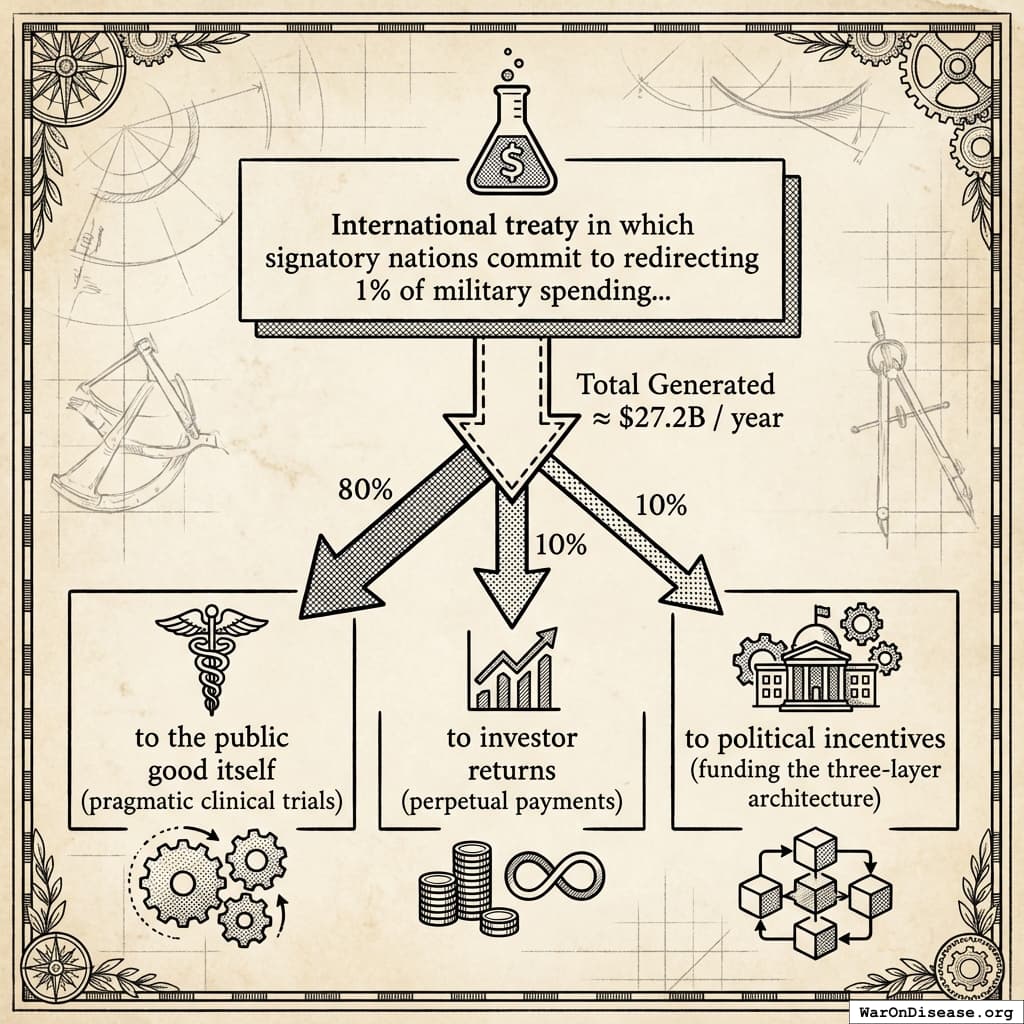
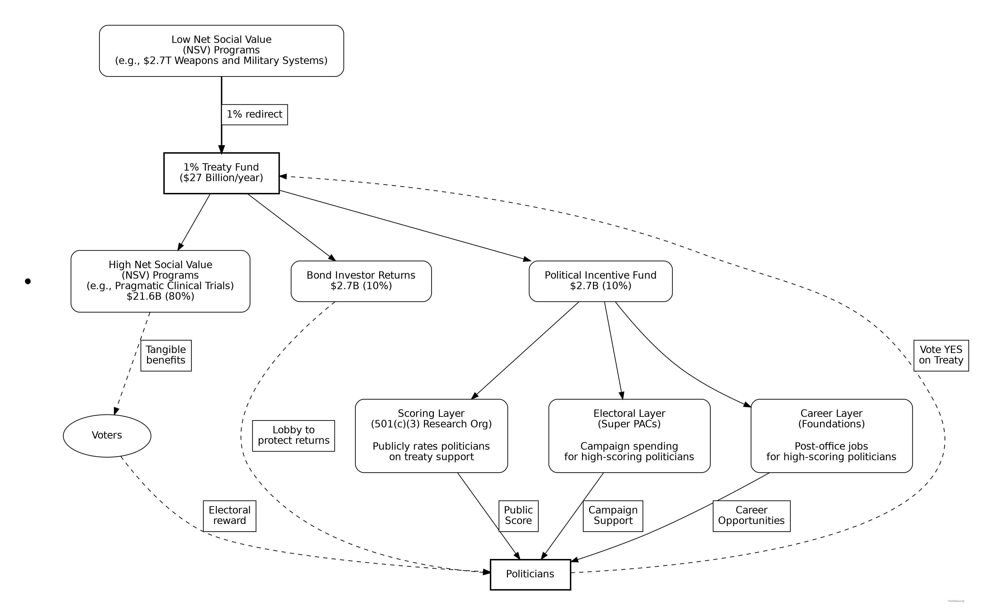
To ground the formal model in concrete terms, consider a hypothetical application. Suppose one’s public goods objective is to simultaneously reduce global conflict and reduce the global burden of disease. Global military expenditure currently exceeds $2.72T annually48, while the global burden of disease exceeds 2.88B DALYs/year (95% CI: 2.63B DALYs/year-3.13B DALYs/year) annually32. An international treaty in which signatory nations commit to redirecting 1% of military spending to a global pragmatic clinical trial system generates approximately $27.2B per year for pragmatic clinical trials, roughly tripling current global clinical trial funding, while creating modest but meaningful pressure toward demilitarization.
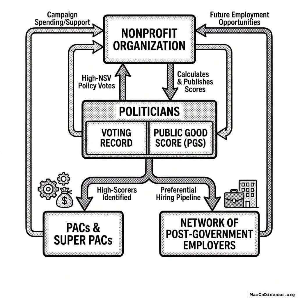
The IAB mechanism for this treaty would allocate treaty inflows as follows:
- 80% to the public good itself (pragmatic clinical trials)
- 10% to investor returns (perpetual payments to those who funded the campaign to pass the treaty)
- 10% to political incentives (funding the three-layer architecture)
This allocation structure creates aligned incentives across all participants. Investors who funded the initial campaign receive perpetual returns ($2.72B annually) as long as the treaty continues, giving them strong incentives to support treaty expansion and defend against repeal. The political incentive allocation ($2.72B annually) funds the three-layer architecture:
Scoring layer: Politicians receive Health Research Scores based on their voting record on treaty ratification, annual funding appropriations, and related legislation. A legislator who votes YES on the treaty and subsequent funding bills sees their score rise; one who votes NO sees their score fall.
Electoral layer: With $2.72B annually available, independent expenditure campaigns can credibly commit: “We will spend $50 million supporting high-scorers in competitive races.” At typical costs per competitive race, this funds meaningful independent campaigns in 20-30 races annually.
Post-office layer: Foundations funded by the political incentive allocation establish eligibility criteria: “The Global Health Leadership Fellowship ($300K/year, 5-year term) requires a career Health Research Score above 70.”
The self-funding nature matters. The treaty’s success generates the resources that sustain both investor returns and political incentives for its continuation and expansion. This creates multiple reinforcing feedback loops:
- Investor pressure for expansion: Investors receiving 10% of $27.2B want the same share of double that (if the treaty expands to 2%), creating a constituency that lobbies for treaty growth
- Political incentives for continuation: Politicians who supported the treaty benefit from ongoing electoral and career support, incentivizing them to defend it against repeal
- Escalation dynamics: Each expansion (1% → 2% → 5%) increases both investor returns and political incentive funding, strengthening the coalition for further expansion
In other words, we’re creating a lobbying machine for public goods that gets stronger the more successful it becomes. This is the same dynamic that made military contractors powerful, except pointed at curing diseases instead of building bombs. Once the flywheel starts spinning, concentrated opposition faces an opponent that grows with every victory.
Consider the decision calculus for a hypothetical Senator Smith facing a vote on treaty ratification:
| Without IABs | With IABs |
|---|---|
| Defense contractors fund opponent if YES | Health Research Score rises 25 points |
| Attack ads: “Smith weakened our military” | Independent campaigns spend $2M supporting Smith |
| Benefits (cures) arrive in 10+ years | Post-office eligibility: Tier 3 → Tier 1 |
| Diffuse beneficiaries cannot coordinate | Expected post-office income: $200K → $400K/yr |
The IAB mechanism transforms the incentive landscape. The concentrated costs (military contractor opposition) remain, but they are now outweighed by concentrated benefits (score increases, electoral support, career advancement). Supporting the treaty becomes the utility-maximizing choice.
3.12 Calibration: Parameter Ranges for Incentive Compatibility
To assess whether IABs can achieve incentive compatibility, we calibrate the model using empirical estimates from campaign finance and lobbying research. Table Table 7 reports parameter ranges.
| Parameter | Symbol | Empirical Range | Source |
|---|---|---|---|
| Defense contractor opposition spending | \(c_i\) | $0.5–5M per race | OpenSecrets 2020 |
| Independent expenditure effect on vote share | \(\epsilon_i\) | 0.5–2 pp per $1M | Spenkuch & Toniatti 2018 |
| Value of 1 pp reelection probability | \(\alpha_i\) | $0.5–2M | Implied by campaign spending |
| Post-office income differential (Tier 1 vs 3) | \(\Delta Y\) | $150–300K/yr | Industry salary data |
| Discount rate for post-office income | \(r\) | 5–10% | Standard |
| Career length post-office | \(T\) | 10–20 years | Empirical average |
Section 3.2 demonstrates that IAB funding levels in the billions can overcome concentrated opposition in the millions, consistent with the “lobbying alpha” asymmetry observed empirically.
4 How IABs Work in Practice
To implement score-dependent payoffs, we need mechanisms. This section specifies a three-layer architecture and analyzes its legality under U.S. law.
4.1 Layer A: Scoring (Data Provision)
An independent entity, structured as a 501(c)(3) research organization, maintains the Public Good Score system.
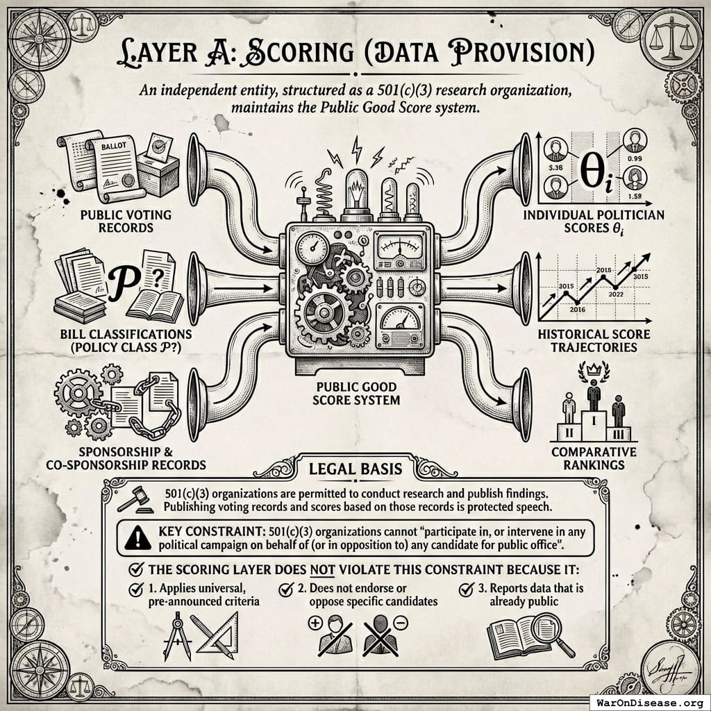
Inputs:
- Public voting records from official government sources
- Bill classifications (does legislation meet criteria for policy class \(\mathcal{P}\)?)
- Sponsorship and co-sponsorship records
Outputs:
- Individual politician scores \(\theta_i\)
- Historical score trajectories
- Comparative rankings
Legal basis: 501(c)(3) organizations are permitted to conduct research and publish findings. Publishing voting records and scores based on those records is protected speech. The key constraint: 501(c)(3) organizations cannot “participate in, or intervene in any political campaign on behalf of (or in opposition to) any candidate for public office”170.
The scoring layer does not violate this constraint because it: 1. Applies universal, pre-announced criteria 2. Does not endorse or oppose specific candidates 3. Reports data that is already public
4.2 Layer B: Electoral Support
Independent actors, structured as 501(c)(4) organizations, PACs, or Super PACs, commit to electoral support rules tied to scores.
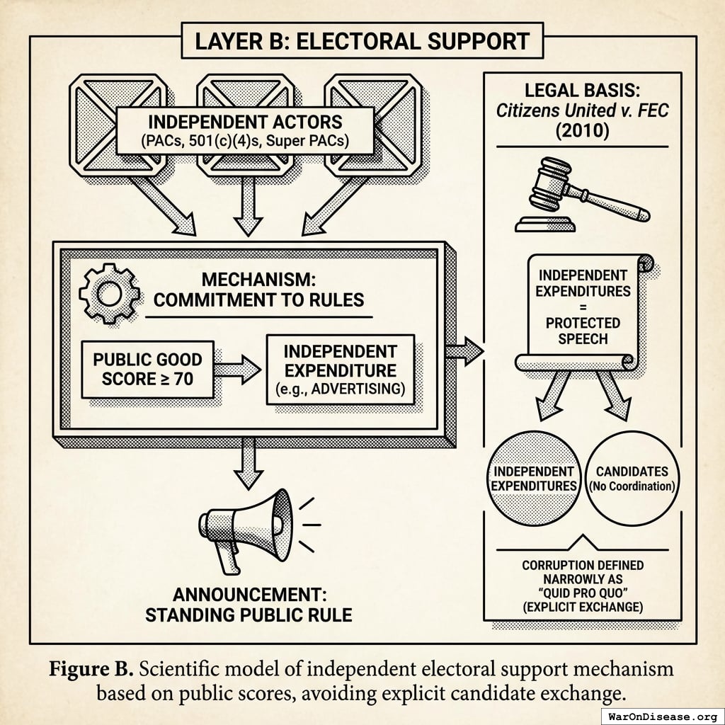
Mechanism:
- Super PACs announce: “We will spend $X million on independent expenditures supporting candidates with Public Good Score ≥ 70 in competitive races”
- This is a standing, public, ex-ante rule, not a deal with any specific candidate
Legal basis: Citizens United v. FEC (2010) held that independent expenditures are protected speech and cannot be limited171. The Court defined corruption narrowly as “quid pro quo,” meaning an explicit exchange of money for official acts. Independent expenditures, not coordinated with candidates, cannot constitute quid pro quo corruption under this standard.
Justice Kennedy wrote that independent spending “does not give rise to corruption or the appearance of corruption” because it is “not prearranged and coordinated” with candidates171. The IAB mechanism satisfies this requirement: support is determined by a public score, not by private arrangements.
4.3 Layer C: Post-Office Benefits
Private foundations, think tanks, and advisory boards establish eligibility criteria tied to scores.
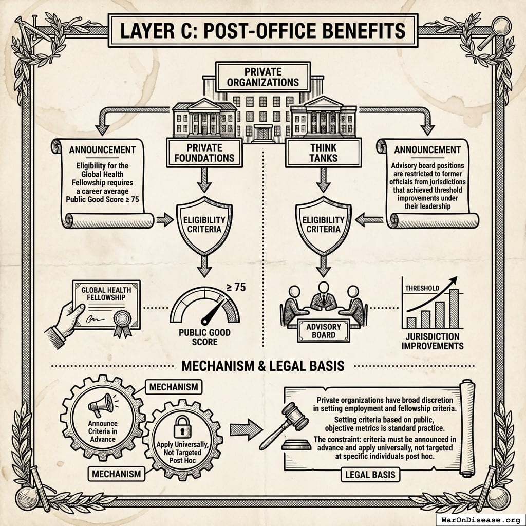
Mechanism:
- Foundations announce: “Eligibility for the Global Health Fellowship requires a career average Public Good Score ≥ 75”
- Think tanks announce: “Advisory board positions are restricted to former officials from jurisdictions that achieved threshold improvements under their leadership”
Legal basis: Private organizations have broad discretion in setting employment and fellowship criteria. Setting criteria based on public, objective metrics is standard practice. The constraint: criteria must be announced in advance and apply universally, not targeted at specific individuals post hoc.
4.4 Why This Is Not Bribery
The legal analysis proceeds through three levels: statutory elements, constitutional protections, and established precedent.
4.4.1 Statutory Analysis: 18 U.S.C. § 201
Under 18 U.S.C. § 201, bribery requires:
- A thing of value given to a public official
- With intent to influence an official act
- As a quid pro quo, a specific exchange172
The IAB mechanism fails each element:
Element 1: No thing of value to officials.
- Scores are information, not things of value. Publishing data about voting records is protected speech.
- Electoral support goes to campaigns, not officials personally. Independent expenditures benefit candidates electorally but are not personal enrichment.
- Post-office opportunities are future employment contingent on (a) leaving office and (b) meeting publicly-announced, universally-applied criteria. Future employment prospects are not “things of value” under bribery law. Otherwise, any industry that hires former regulators would be guilty of bribery.
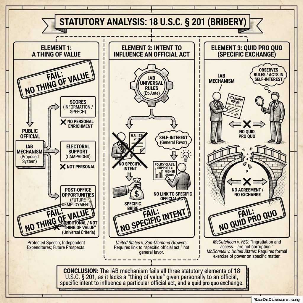
Element 2: No specific intent to influence.
Rules are universal and ex-ante. No one tells any official “vote for X and receive Y.” The rule is: “Any official who supports this class of policies will score higher.” This is categorically different from “I will give you money if you vote yes on H.R. 1234.”
The distinction matters legally. In United States v. Sun-Diamond Growers173, the Supreme Court held that illegal gratuities require a link to a “specific official act,” not merely a general desire to curry favor. IABs create no such link; they reward policy classes, not specific votes.
Element 3: No quid pro quo.
No exchange occurs with any official. Officials are not party to any agreement. They merely observe standing rules and act in their self-interest. The Supreme Court in McCutcheon v. FEC174 held that “ingratiation and access… are not corruption” and that only “quid pro quo corruption” justifies regulation of political speech.
McDonnell v. United States (2016) further narrowed the definition of “official act,” requiring a formal exercise of governmental power on a specific matter175. The IAB mechanism does not pay for specific official acts; it creates a scoring system that independent actors may choose to use.
4.4.2 Constitutional Protections
The IAB architecture is protected by the First Amendment at multiple levels:
- Scoring layer: Publishing voting records and scores based on those records is core political speech. The government cannot prohibit citizens from evaluating and publicizing legislators’ voting records.

Electoral layer: Citizens United held that independent expenditures are protected speech. The government cannot limit spending by independent actors to support or oppose candidates based on their policy positions.
Post-office layer: Private organizations have First Amendment associational rights to set their own membership and employment criteria. A foundation requiring fellows to have supported certain policies is no different from a think tank preferring scholars who share its intellectual orientation.
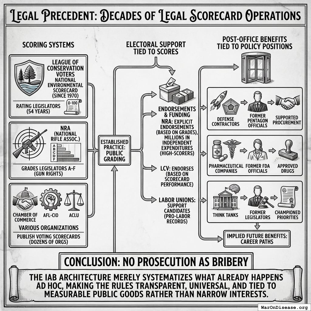
4.4.3 Established Precedent: Decades of Legal Scorecard Operations
The most powerful evidence that IABs are legal is that their core components have operated openly for decades without prosecution:
Scoring systems:
- The League of Conservation Voters has published its National Environmental Scorecard since 1970, for 54 years rating legislators on environmental votes
- The NRA grades legislators A through F on gun rights votes and publicizes the ratings
- The Chamber of Commerce, AFL-CIO, ACLU, and dozens of other organizations publish voting scorecards
Electoral support tied to scores:
- The NRA explicitly endorses candidates based on their grades and spends millions on independent expenditures supporting high-scorers
- The LCV endorses based on scorecard performance
- Labor unions support candidates with pro-labor voting records
Post-office benefits tied to policy positions:
- Defense contractors hire former Pentagon officials who supported procurement programs
- Pharmaceutical companies hire former FDA officials who approved their drugs
- Think tanks hire former legislators who championed their policy priorities
None of these activities have been prosecuted as bribery. The IAB architecture merely systematizes what already happens ad hoc, making the rules transparent, universal, and tied to measurable public goods rather than narrow interests.
4.4.4 The Key Legal Distinction
Bribery corrupts official judgment by introducing private benefit that conflicts with public duty. IABs align private benefit with public duty, rewarding officials for doing their job well as measured by policy outcomes. This is the opposite of corruption.
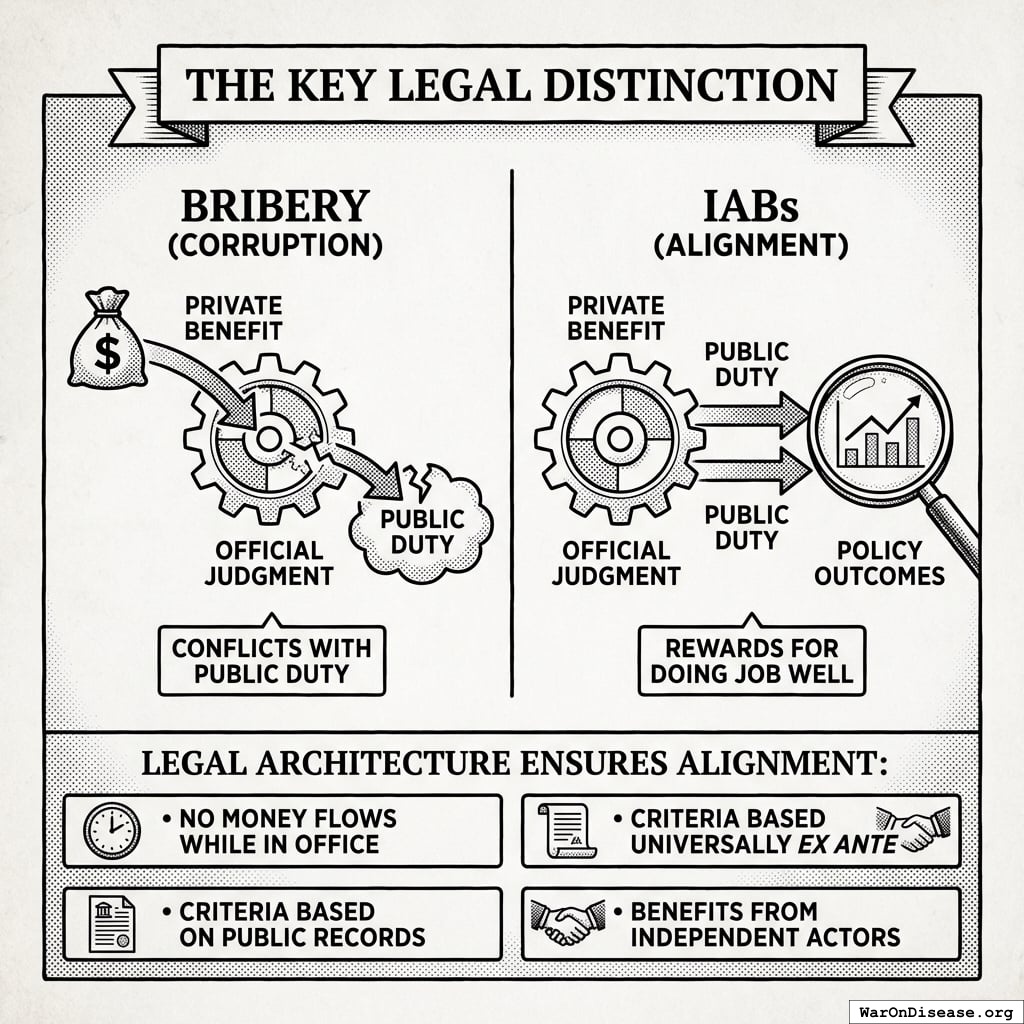
The legal architecture ensures this alignment holds:
- No money flows to officials while in office
- Rules apply universally to all officials ex ante
- Criteria are based on public records, not private arrangements
- Benefits come from independent actors, not parties to any agreement with officials
4.5 Legal Entity Separation
| Layer | Entity Type | Permitted Activities | Prohibited Activities |
|---|---|---|---|
| Scoring | 501(c)(3) | Research, publish scores | Campaign intervention |
| Electoral | 501(c)(4), PAC, Super PAC | Independent expenditures | Coordination with candidates |
| Post-office | Private foundations | Set eligibility criteria | Condition grants on specific votes |
4.6 Funding Sources and Foundation Investment
IABs can attract capital from multiple sources with different legal constraints.
Commercial investors (impact funds, family offices, institutional capital) face no restrictions on which layers they fund. If the bond offers market-rate or above-market returns, commercial capital can fund all activities, including the electoral layer.
Private foundations seeking to invest via Program-Related Investments (PRIs) face an additional constraint. IRS regulations require that PRIs not be used “directly or indirectly to lobby or for political purposes”170. This means:
| Layer | Foundation PRI Eligible? | Notes |
|---|---|---|
| Scoring | Yes | Pure research/data |
| Electoral | No | Explicitly political |
| Post-office | Yes | Employment criteria |
This constraint is less significant than it appears. In a unified bond offering, the allocation happens after policy success. Investors receive returns from policy revenue, which is then allocated across uses. Foundations investing via PRI could have their returns earmarked for non-electoral uses.
Precedent: The Rockefeller Foundation invested in the Peterborough Social Impact Bond via PRI. The Kresge Foundation and Living Cities provided junior tranches in Massachusetts Pay for Success projects. Bloomberg Philanthropies guaranteed Goldman Sachs’ investment in the Rikers Island SIB. Foundation participation in outcome-based bonds is established practice.
Practical implication: For IABs offering strong commercial returns, foundation PRIs are a supplementary funding source, not a necessity. The electoral layer, the one foundations cannot fund, can be capitalized by return-seeking investors.
5 What Could Go Wrong
5.1 Gaming and Metric Corruption
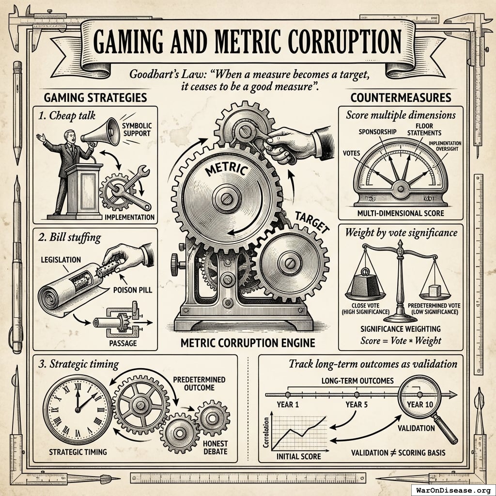
Any metric can be gamed. Goodhart’s Law states: “When a measure becomes a target, it ceases to be a good measure”176. Potential gaming strategies:
- Cheap talk: Politicians vote symbolically for popular positions but undermine implementation
- Bill stuffing: Attach poison pills to supported legislation
- Strategic timing: Time votes when outcomes are predetermined
Countermeasures:
- Score multiple dimensions (votes, sponsorship, floor statements, implementation oversight)
- Weight by vote significance (close votes count more)
- Track long-term outcomes as validation (though not as scoring basis)
5.2 Plutocracy Objection and the “Lobbying With Extra Steps” Critique
The most serious criticism economists are likely to raise: “This is just lobbying with extra steps. You’re creating a well-funded interest group to lobby politicians for your preferred policies.”
This criticism deserves a careful response, as it goes to the heart of whether IABs represent genuine institutional innovation or merely repackage existing capture dynamics.
What makes IABs structurally different from corporate lobbying:
Comparative welfare criterion: IABs fund reallocation from \(NSV_{source} < NSV_{target}\) programs. Corporate lobbying seeks absolute budget increases for the lobbying firm’s industry, regardless of comparative value. Defense contractors lobby for more military spending without specifying what gets cut. IABs specify both the source (lower-NSV) and target (higher-NSV), creating a welfare-improving constraint.
Public good vs. private good alignment: Corporate lobbying aligns politician incentives with excludable private benefits (military contracts flow to specific firms). IAB-supported policies produce non-excludable public goods (cures, climate stability). Investors cannot capture the primary benefits. They accrue to the general public. Investors capture only a fraction of the funding flow, not the end-state benefit.
Transparent, universal, ex-ante rules: Corporate lobbying operates through opaque relationships (revolving door promises, implicit quid pro quos, insider access). IABs publish scoring criteria ex-ante, apply them universally to all politicians regardless of relationship, and make scores publicly available. Any politician can improve their score through observable actions.
Diffuse vs. concentrated funders: Corporate lobbying concentrates returns to a small number of firms. IABs, if structured as retail-accessible securities, allow millions of diffuse beneficiaries to invest small amounts. A $1,000 IAB investment makes a retiree a “special interest” in pragmatic clinical trials, structurally impossible with current lobbying.
Metric validation: Corporate lobbying success is measured by dollars flowing to the lobbying firm. IAB success is measured by rigorous external benefit-cost analyses (Copenhagen Consensus, GiveWell, academic literature). The scoring organizations are independent 501(c)(3) entities, not the investors themselves.
However, the objection retains force: IABs do not democratize power; they redirect it. Whose conception of “public good” defines the NSV ranking? What prevents IAB funders from capturing the scoring process? What prevents redirected resources from being recaptured by new concentrated interests?
The structural answer: The four-layer governance stack (Section 6) addresses these concerns. Layer 0 (Wishocracy for Domain Ranking) democratizes which domains receive funding via citizen pairwise comparisons aggregated with expert BCR data. Layer 2 (Wishocracy for Within-Domain Allocation) democratizes allocation within approved domains. Random pairwise sampling makes advertising economically infeasible (~0.1% appearance probability per campaign → $200M cost to shift rankings → cheaper to just do the research). IABs (Layer 1) solve only the adoption problem: getting politicians to vote for reallocation. Democratic legitimacy is addressed at Layers 0 and 2, not Layer 1.
5.3 Unintended Consequences
Political systems are complex. Possible unintended consequences:
- Crowding out intrinsic motivation: If politicians come to see policy support as instrumental, they may become more transactional overall
- Metric fixation: Excessive focus on scored policies at the expense of unscored but important issues
- Legitimacy erosion: Public perception that politicians are “bought” (even legally) may reduce trust
These concerns warrant monitoring, but must be weighed against the status quo: 55.0M deaths/year (95% CI: 46.6M deaths/year-63.2M deaths/year) annually from diseases that faster research could address, while $2.72T flows to military spending with 0.6x (95% CI: 0.4x-0.9x) ROI. The unintended consequences of inaction, continued optimization of government spending for lobbying intensity rather than human welfare, dwarf any plausible risk from making pro-health votes more rewarding. Politicians are already transactional; IABs redirect that transactionality toward public goods.
6 Where IABs Fit in Democratic Reform
6.1 The Four-Layer Governance Stack
IABs address one specific failure mode: how to get welfare-improving policies adopted when concentrated interests oppose them. They fit within a broader governance stack:
- Layer 0 (Domain Ranking): Expert organizations (Copenhagen Consensus, GiveWell, IMF) provide benefit-cost data; citizens aggregate via pairwise comparisons to produce democratic domain rankings with capture-resistant legitimacy.
- Layer 1 (IABs): Insert rankings into politician utility functions via score-dependent electoral support and career benefits. This is the binding constraint and the focus of this paper.
- Layer 2 (Within-Domain Allocation): Once resources are redirected, mechanisms like aggregated pairwise preference allocation177 prevent capture by new concentrated interests.
- Layer 3 (Project Selection): Domain-specific marketplaces (prediction markets, prize markets, retroactive public goods funding) allocate to specific projects.
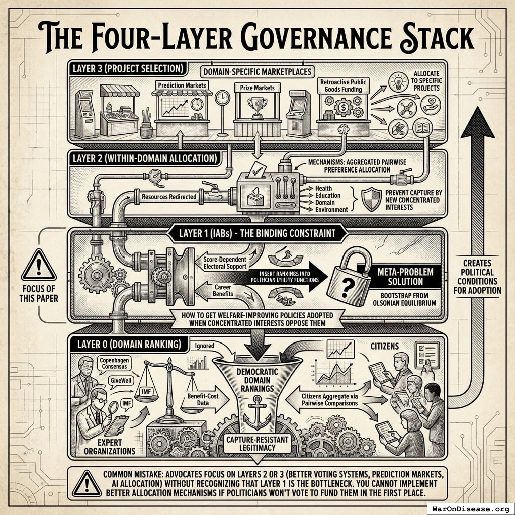
Layer 0 rankings exist but are ignored because they don’t appear in politician utility functions. Layers 2-3 cannot function until Layer 1 creates the political conditions for their adoption.
Common mistake: Advocates focus on Layers 2 or 3 (better voting systems, prediction markets, AI allocation) without recognizing that Layer 1 is the bottleneck. You cannot implement better allocation mechanisms if politicians won’t vote to fund them in the first place. IABs solve the meta-problem: how to bootstrap from the current Olsonian equilibrium to one where better governance mechanisms can be adopted.
6.2 Comparison to Alternative Governance Mechanisms
Table 9 compares IABs to alternative governance reform approaches. Comparison criteria: feasibility assessments, implementation timelines, capital requirements, and structural barriers. The analysis draws on historical precedents for institutional reform, capital requirements relative to available funding sources, political economy barriers, and adoption rates of analogous mechanisms.
| Approach | Feasibility Assessment | Time Horizon | Capital Required | Key Barrier | What It Solves |
|---|---|---|---|---|---|
| IABs | Moderately challenging | Medium-term (10-20 years) | $200M-$500M initial | Bootstrap funding | Adoption of welfare-improving policies |
| Wishocracy (post-IAB) | Moderate (conditional on IABs)* | Medium-term (5-10 years) | $50M-$200M | Requires treaty first | Post-adoption allocation |
| Futarchy (prediction markets) | Very challenging | Long-term (15-25 years) | $100M-$500M | Manipulation, adoption | Policy → outcome mapping |
| Quadratic Voting/Funding | Very challenging | Long-term (10-20 years) | $50M-$200M | Constitutional barriers | Preference intensity |
| Optimocracy (algorithmic governance) | Moderate (private); Challenging (gov’t) | Near-term (1-2 years private); Medium-term (5-15 years gov’t) | $10M-$100M (private DAO); $500M+ (gov’t adoption) | Goodhart’s Law, oracle capture | Removes political discretion for routine allocation |
| Charter Cities | Very challenging | Very long-term (20-40 years) | $1B+ | Sovereignty, scale | Competitive governance |
| NSV Ranking Alone | Infeasible | N/A | $10M-$50M | No incentive linkage | Information (ignored) |
*Wishocracy becomes feasible only after IABs create political conditions for resource reallocation; otherwise faces same adoption barriers as IABs.
Other governance mechanisms:
Algorithmic governance (Optimocracy) faces capture at the design level: whoever controls the algorithm specification controls outcomes. However, this can be mitigated through constitutional-level metric selection (via Wishocracy), decentralized oracles, and smart contract enforcement. See the Optimocracy paper for detailed mechanism design addressing these challenges.
Futarchy (prediction markets for policy) is intellectually elegant but faces adoption barriers. Who decides the outcome metrics? How do you prevent market manipulation? IABs could bootstrap futarchy by making politicians willing to adopt prediction-market-based governance.
Charter cities / competitive governance avoid the adoption problem (exit rather than voice) but face scale and sovereignty constraints.
NSV rankings alone are infeasible because they lack incentive linkage. The empirical fact motivating this entire paper.
A parallel + sequenced implementation strategy:
- Immediate (0-2 years): Deploy private Optimocracy DAO for philanthropic/investment capital allocation; no government permission required. Simultaneously begin IAB development.
- Near-term (2-10 years): IABs for high-value domains (health, climate, pandemic preparedness). Private Optimocracy scales and demonstrates superior outcomes.
- Medium-term (10-20 years): Use IAB political capital + Optimocracy track record to pass government pilots for Wishocracy and Optimocracy.
- Long-term (20+ years): Hybrid Wishocracy-Optimocracy architecture becomes standard for capture-resistant governance.
Optimocracy and IABs can develop in parallel. Private Optimocracy doesn’t require government adoption, so it can demonstrate proof-of-concept while IABs work on the political adoption problem.
6.3 What IABs Do Not Solve
IABs solve the adoption problem (the binding constraint) but not the complete resource allocation problem. The four-layer stack (Section 6.1) addresses domain ranking, within-domain allocation, and project selection through complementary mechanisms.
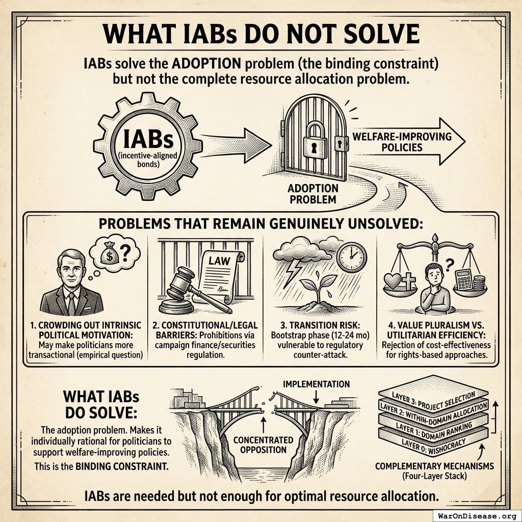
Problems that remain genuinely unsolved:
- Crowding out intrinsic political motivation: IABs may make politicians more transactional (empirical question requiring evaluation)
- Constitutional/legal barriers: Some jurisdictions may prohibit IAB mechanisms via campaign finance or securities regulation
- Transition risk: Bootstrap phase (12-24 months before proof-of-concept) vulnerable to regulatory counter-attack
- Value pluralism vs. utilitarian efficiency: Even with Wishocracy at Layer 0 allowing citizens to weight domains by their values, some citizens may reject the entire framework of cost-effectiveness analysis in favor of deontological or rights-based approaches
What IABs do solve: The adoption problem. They make it individually rational for politicians to support welfare-improving policies despite concentrated opposition. This is the binding constraint in the governance stack. Without solving adoption, better allocation mechanisms (Layers 2-3) cannot be implemented. IABs are needed but not enough for optimal resource allocation.
7 Beyond Health: Climate, Nuclear Risk, and More
The IAB architecture is not specific to health policy. It applies to any global coordination problem satisfying three conditions:
- Measurable outcomes: There exists a metric politicians can be scored on
- Political control: Politicians’ actions (votes, treaties, budget allocations) affect outcomes
- Diffuse benefits, concentrated costs: The Olsonian collective action failure applies
These conditions identify domains where the mechanism design approach is applicable. The formal requirements (A1–A5) must be satisfied, with domain-specific adaptations to the scoring function \(f\) and payoff calibration.
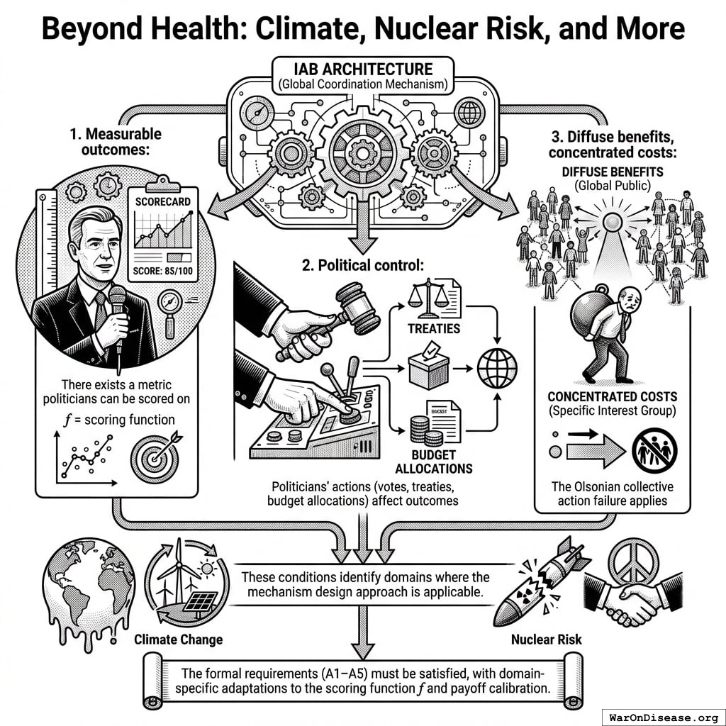
7.1 The General Template
Any global public good satisfying the above conditions can be “IAB-ified” using the structure in Table 10.
| Component | Function | Legal Form |
|---|---|---|
| Metric | Measures politician-controlled outcomes | Defined by 501(c)(3) research org |
| Score | Translates actions into public number | Published by independent body |
| Electoral layer | Rewards high-scorers with campaign support | 501(c)(4), PAC, Super PAC |
| Post-office layer | Reserves prestige positions for high-scorers | Foundations, think tanks |
7.2 Candidate Domains
We briefly survey three domains where IABs are applicable; Appendix B provides detailed specifications.
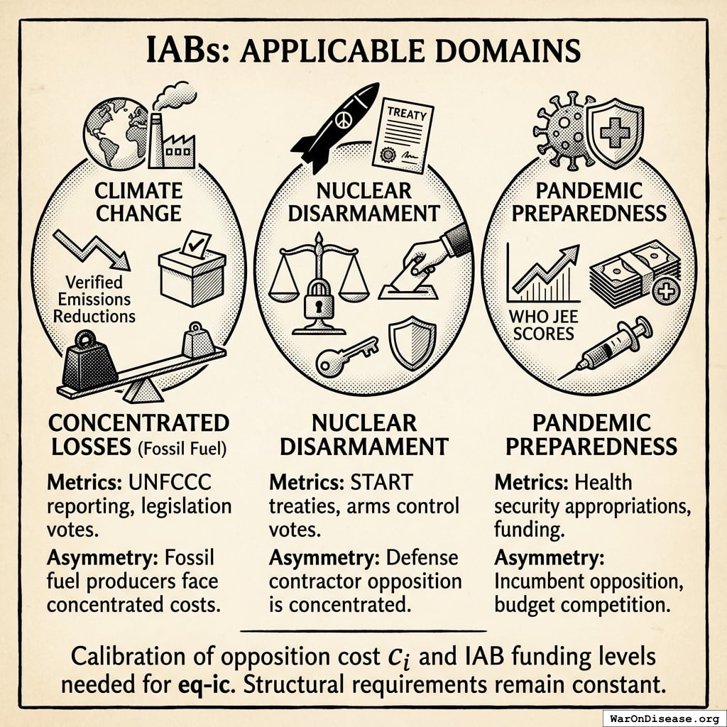
Climate change. Verified emissions reductions (UNFCCC reporting) provide a measurable metric. Politicians can be scored on climate legislation votes, treaty ratification, and budget allocations. The concentrated-diffuse asymmetry is stark: fossil fuel producers face concentrated losses while climate benefits are globally diffuse.
Nuclear disarmament. Verified warhead reductions under START-type treaties provide objective metrics. The scoring function would weight votes on arms control treaties, military authorization amendments, and non-proliferation funding. Defense contractor opposition creates concentrated costs; security benefits are diffuse.
Pandemic preparedness. WHO Joint External Evaluation scores and pandemic preparedness funding levels are measurable. Health security appropriations votes provide a scoring basis. Pharmaceutical incumbent opposition and budget competition create concentrated resistance; pandemic prevention benefits the global population.
Each domain requires calibration of the opposition cost \(c_i\) and the IAB funding levels needed to satisfy Equation 16. The structural requirements remain constant across applications.
7.3 Welfare Accounting of the IAB Mechanism
The paper demonstrates that IABs redirect resources from low-NSV to high-NSV programs, but economists will correctly ask: what is the net welfare impact accounting for the mechanism’s own costs?
Mechanism costs (annual, steady-state):
| Component | Estimated Annual Cost | Purpose |
|---|---|---|
| Scoring organizations | $10M-$50M | Research, data, scoring methodology |
| Independent expenditure campaigns | $100M-$500M | Electoral support for high-scorers |
| Post-office foundations | $50M-$200M | Fellowships, advisory positions |
| Total mechanism overhead | $160M-$750M/year | Ongoing operation |
Benefits (illustrative, 1% military reallocation treaty):
| Benefit Category | Estimated Annual Value | Source |
|---|---|---|
| Peace dividend (reduced conflict costs) | 1% × $11.4T (95% CI: $9.01T-$14.1T) global war costs | |
| Pragmatic clinical trials acceleration | $27.2B reallocated × 4.75 BCR | |
| Total annual benefits | $172B (95% CI: $140B-$213B) | Conservative estimate |
Net welfare calculation:
Net Societal Value = Benefits - Costs = $172B (95% CI: $140B-$213B) - $750M (95% CI: $160M-$750M) ≈ $172B (95% CI: $140B-$213B)/year (costs are <1% of benefits).
Benefit-cost ratio of the IAB mechanism itself:
\[ \begin{gathered} BCR_{IAB} = \frac{Benefit_{peace+RD}}{Cost_{IAB,ann}} = \frac{\$172B}{\$750M} = 230 \\[0.5em] \text{where } Benefit_{peace+RD} \\ = Benefit_{peace,soc} + Benefit_{RD,ann} \\ = \$114B + \$58.6B \\ = \$172B \\[0.5em] \text{where } Benefit_{peace,soc} \\ = Cost_{war,total} \times Reduce_{treaty} \\ = \$11.4T \times 1\% \\ = \$114B \\[0.5em] \text{where } Cost_{war,total} \\ = Cost_{war,direct} + Cost_{war,indirect} \\ = \$7.66T + \$3.7T \\ = \$11.4T \\[0.5em] \text{where } Cost_{war,direct} \\ = Loss_{life,conflict} + Damage_{infra,total} \\ + Disruption_{trade} + Spending_{mil} \\ = \$2.45T + \$1.88T + \$616B + \$2.72T \\ = \$7.66T \\[0.5em] \text{where } Loss_{life,conflict} \\ = Cost_{combat,human} + Cost_{state,human} \\ + Cost_{terror,human} \\ = \$2.34T + \$27B + \$83B \\ = \$2.45T \\[0.5em] \text{where } Cost_{combat,human} \\ = Deaths_{combat} \times VSL \\ = 234{,}000 \times \$10M \\ = \$2.34T \\[0.5em] \text{where } Cost_{state,human} \\ = Deaths_{state} \times VSL \\ = 2{,}700 \times \$10M \\ = \$27B \\[0.5em] \text{where } Cost_{terror,human} \\ = Deaths_{terror} \times VSL \\ = 8{,}300 \times \$10M \\ = \$83B \\[0.5em] \text{where } Damage_{infra,total} \\ = Damage_{comms} + Damage_{edu} + Damage_{energy} \\ + Damage_{health} + Damage_{transport} \\ + Damage_{water} \\ = \$298B + \$234B + \$422B + \$166B + \$487B + \$268B \\ = \$1.88T \\[0.5em] \text{where } Disruption_{trade} \\ = Disruption_{currency} + Disruption_{energy} \\ + Disruption_{shipping} + Disruption_{supply} \\ = \$57.4B + \$125B + \$247B + \$187B \\ = \$616B \\[0.5em] \text{where } Cost_{war,indirect} \\ = Damage_{env} + Loss_{growth,mil} \\ + Loss_{capital,conflict} + Cost_{psych} \\ + Cost_{refugee} + Cost_{vet} \\ = \$100B + \$2.72T + \$300B + \$232B + \$150B + \$200B \\ = \$3.7T \\[0.5em] \text{where } Benefit_{RD,ann} \\ = Spending_{trials} \times Reduce_{pct} \\ = \$60B \times 97.7\% \\ = \$58.6B \\[0.5em] \text{where } Reduce_{pct} \\ = 1 - \frac{Cost_{pragmatic,pt}}{Cost_{P3,pt}} \\ = 1 - \frac{\$929}{\$41K} \\ = 97.7\% \end{gathered} \]
Even using the high-end cost estimate ($750M (95% CI: $160M-$750M)) and conservative benefits (ignoring climate, pandemic preparedness, other applications), the mechanism’s BCR exceeds 230:1 (95% CI: 186:1-284:1). The overhead cost is <1% of benefits, comparable to the expense ratio of efficient index funds (0.03-0.3%).
Sensitivity to failure risk:
If the mechanism has only a 10% chance of achieving treaty passage, expected BCR falls to ~23:1, still dramatically positive. If success probability is 50%, expected BCR is ~115:1. The mechanism justifies its costs across a wide range of success probabilities.
Comparison to alternative governance reforms:
| Reform Mechanism | Estimated Annual Cost | Estimated Benefits | BCR |
|---|---|---|---|
| IABs (this paper) | |||
| Layer 0 only (Wishocracy domain ranking without Layer 1) | $10M-$50M | ~$0 (ignored by politicians) | 0:1 |
| Futarchy infrastructure | $500M-$1B | Uncertain | Unknown |
| Charter cities | $1B+ | Limited scale | 1:1 to 5:1 |
IABs’ welfare accounting is favorable precisely because they solve the adoption problem. Better domain prioritization (Layer 0 Wishocracy) costs little but achieves nothing if politicians ignore the rankings. Better allocation mechanisms (futarchy, Layer 2 Wishocracy) are valuable only if adopted, which requires Layer 1 (IABs) first. The mechanism’s overhead is justified by making all other governance improvements politically feasible.
Risks to welfare accounting:
- Crowding out intrinsic motivation: If IABs make politicians more transactional, could reduce welfare from unscored policies
- Capture of scoring process: Layer 0 (Wishocracy for Domain Ranking) mitigates this by requiring capture of ALL expert organizations AND manipulation of millions of citizen preferences
- Regulatory backlash costs: Legal battles and reputation damage if mechanism is perceived as illegitimate
Even accounting for these risks, the net welfare impact remains strongly positive (BCR > 200:1).
7.3.1 Sensitivity Analysis of Mechanism BCR
The benefit-cost ratio calculation above uses point estimates. The following Monte Carlo analysis propagates uncertainty through all input parameters to show the full distribution of possible outcomes.
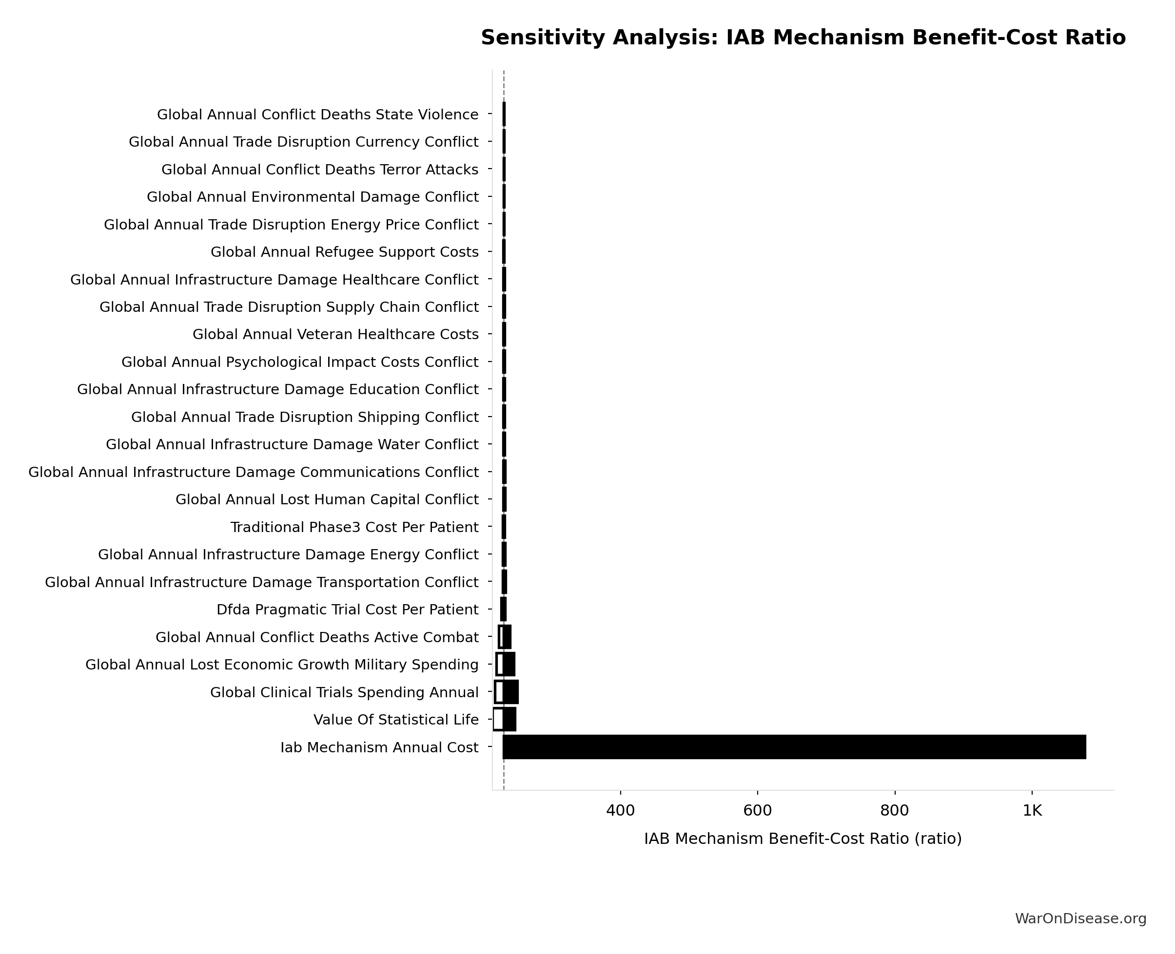
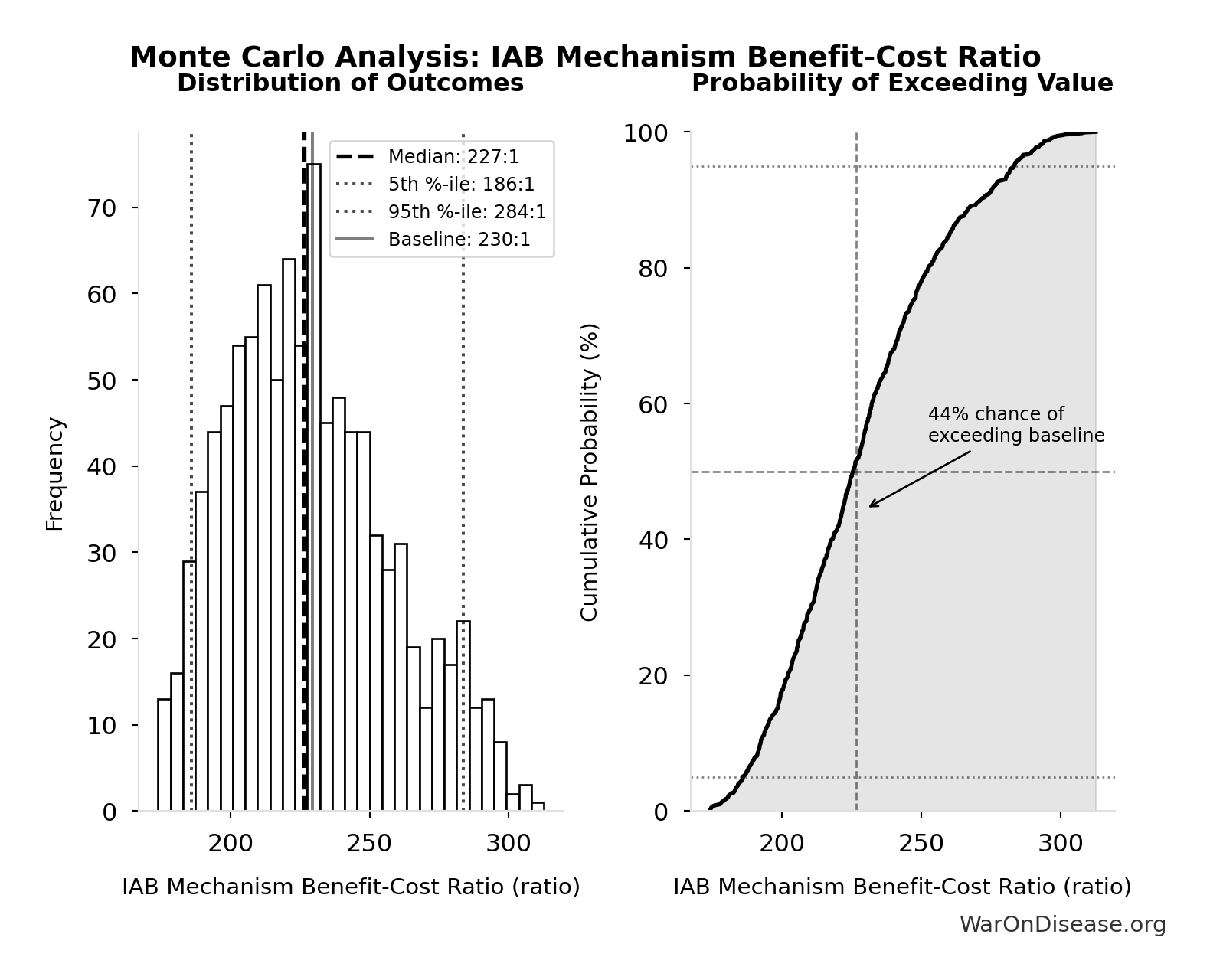
Simulation Results Summary: IAB Mechanism Benefit-Cost Ratio
| Statistic | Value |
|---|---|
| Baseline (deterministic) | 230:1 |
| Mean (expected value) | 229:1 |
| Median (50th percentile) | 227:1 |
| Standard Deviation | 29.6:1 |
| 90% Confidence Interval | [186:1, 284:1] |
The histogram shows the distribution of IAB Mechanism Benefit-Cost Ratio across 10,000 Monte Carlo simulations. The CDF (right) shows the probability of the outcome exceeding any given value, which is useful for risk assessment.
The Monte Carlo results confirm that the mechanism’s BCR remains strongly positive across the full range of parameter uncertainty. Even at the 5th percentile (worst-case), the BCR exceeds 186:1, indicating robust welfare gains regardless of which parameter values materialize.
8 Conclusion
Incentive Alignment Bonds represent a new application of mechanism design to democratic governance. By making support for public-good policies incentive-compatible for utility-maximizing politicians, IABs address the collective action failure identified by Olson: concentrated interests systematically defeating diffuse interests in political competition.
The contribution is fivefold:
Theoretical: We formalize political incentive alignment as a mechanism design problem, provide explicit functional forms for politician utility components, and prove conditions for incentive compatibility.
Empirical: We provide numerical calibration demonstrating that the incentive compatibility condition is achievable with realistic parameters in selected domains (pandemic preparedness, health research) while showing mechanism failure in high-opposition domains (defense reallocation) absent enough funding.
Instrumental: We define IABs through three primitive properties: investor alignment, politician alignment, and funding from lower-value sources. Together, these create a self-sustaining mechanism for public good production that restores alignment between politician incentives and general welfare.
Practical: We specify a three-layer architecture (scoring, electoral, post-office) that achieves alignment without violating anti-bribery law, and demonstrate that the bootstrap problem is solvable due to ROI economics and capital asymmetry.
Welfare-Economic: We provide a comparative criterion (\(NSV_{source} < NSV_{target}\)) for identifying appropriate funding sources, implying a natural ranking of expenditures by marginal social value. We demonstrate why specified reallocation, rather than budget addition, is needed to achieve real resource shifts under soft budget constraints. Welfare accounting shows the mechanism itself has a BCR of 230:1 (95% CI: 186:1-284:1), justifying overhead costs across a wide range of success probabilities.
Important limitations remain. Gaming and metric corruption require ongoing institutional vigilance. The plutocracy objection, that wealthy funders determine priorities, is addressed structurally by Wishocracy (Layer 2), which democratizes allocation decisions via aggregated citizen preferences and prevents advertising-based capture through random pairwise sampling. The capital asymmetry ($454T household wealth vs. $5T concentrated interests) combined with retail-accessible securities ensures that funding itself becomes democratized. Unintended consequences on political culture (e.g., crowding out intrinsic motivation) remain empirical questions requiring pilot evaluation. These considerations counsel for careful pilot implementation with rigorous evaluation before scaling.
8.1 The Bootstrap Problem and Regulatory Resistance
The biggest challenge is political: concentrated interests threatened by IABs will attempt to regulate them out of existence before they can demonstrate effectiveness.
If IABs successfully redirect even 1% of military spending ($27.2B globally), military contractors will face real losses. They will deploy their existing lobbying infrastructure to ban, restrict, or capture the mechanism. Potential regulatory attacks include:
- Campaign finance regulation: Classify IAB-funded independent expenditures as illegal coordination
- Securities regulation: Prohibit retail investment in “political outcome bonds”
- Tax law changes: Eliminate tax-exempt status for scoring organizations
- Capture attempts: Lobby to control the scoring methodology or install friendly board members
The bootstrap paradox: IABs need enough scale to create political incentives strong enough to resist regulatory capture, but concentrated interests will attempt to kill the mechanism before it reaches that scale. It’s the classic Catch-22: you need to be big enough to win, but your enemies will try to kill you while you’re small.
Potential solutions:
- First-mover advantage in permissive jurisdictions: Pilot in countries with strong free speech protections and established independent expenditure precedent (U.S., UK)
- Rapid scaling: Achieve critical mass ($200M-$2B deployed) within 18-24 months, before regulatory counter-mobilization
- Constitutional protection: Establish that IAB mechanisms fall under protected political speech (U.S. First Amendment, European Convention on Human Rights Article 10)
- Diverse funding sources: Avoid dependence on any single capital source that could be regulated
- International treaty protection: Once a treaty is adopted, signatories have incentive to protect the mechanism that secured their score-improvement
The mechanism’s survival likely depends on achieving proof-of-concept success (one treaty ratified) before incumbent industries can coordinate effective regulatory opposition. This creates a premium on execution speed and strategic sequencing of target domains.
Why the Initial Fundraising Challenge is Solvable: Capital Asymmetry and ROI
Raising the first $200M-$500M (Phase 1 of the $1B campaign) before concentrated interests mobilize counter-lobbying appears daunting until we consider two factors: (1) the massive ROI potential and (2) the capital asymmetry favoring diffuse beneficiaries.
ROI makes initial funding rational for risk-tolerant capital:
As shown in Section 2.1, the expected ROI economics make early investment rational: conditional annual ROI of 272% upon treaty passage, with perpetual revenue streams. Even with high risk and long timelines, the asymmetric upside makes initial funding economically rational, not philanthropic. This changes the bootstrap calculus: early investors are not donors making grants; they are rational actors making high-risk, high-return investments.
Capital asymmetry ensures scalability beyond Phase 1:
Phase 1 requires $200M-$500M to demonstrate traction, which is small relative to the aggregate capital available to diffuse beneficiaries:
- Concentrated opposition (military contractors, fossil fuel companies): $5T market cap, spending $100M-$1B/year on lobbying
- Diffuse beneficiaries (everyone who benefits from cures, climate stability): $454T household wealth (Section 2.3)
The 90:1 capital advantage means that even if concentrated interests attempt counter-lobbying, they face a resource constraint. If military contractors allocate $500M to kill IABs, diffuse beneficiaries can deploy $5B in response, and still represent only 0.001% of available household wealth. The political change ROI (100-10,000x) that military contractors exploit becomes accessible to millions of retail investors.
Empirical precedent: Cryptocurrencies raised $30B+ in ICOs (2017-2018) with far weaker value propositions than 272% conditional ROI backed by lobbying economics. Green bonds reached $500B outstanding by 2023. If IABs can be structured as retail-accessible securities, the capital mobilization problem is not “can we raise $1B?” but “can we structure the offering legally?”
The race condition: Concentrated interests can mobilize regulatory opposition within 12-24 months of IAB visibility. But if: 1. Phase 1 ($200M-$500M) is raised from high-risk capital (impact funds, crypto whales, patient billionaires) 2. Rapid deployment achieves measurable traction (one scoring cycle, measurable electoral impact) 3. Momentum builds (even partial progress increases bond value through demonstrated efficacy) 4. Retail offering opens to millions of diffuse beneficiaries for the remaining campaign funding
…then the mechanism reaches escape velocity before regulatory capture becomes feasible. Defense contractors cannot outspend $50B+ in mobilized retail capital without bankrupting themselves.
Conclusion: The initial fundraising challenge is solvable because (a) ROI economics make early investment rational for risk-tolerant capital, and (b) capital asymmetry ensures that once traction is demonstrated, scaling capital to the full $1B exceeds any plausible counter-lobbying budget. The binding constraint is execution speed, not capital availability.
Future research should address several open questions: What scoring mechanisms are most robust to gaming? How do IABs interact with existing campaign finance institutions? What governance structures best prevent capture of the scoring layer? Can IABs be adapted to non-democratic political systems? What legal strategies best protect the mechanism from regulatory attack? Empirical testing, beginning with single-issue pilot implementations, will be essential to validate the theoretical framework presented here.
If IABs can change political behavior at scale, if they can make supporting measurable public goods the career-maximizing choice for politicians, the architecture becomes available for climate, nuclear risk, pandemic preparedness, and every domain where humanity’s long-term welfare depends on overcoming collective action failures. The mechanism does not require politicians to become better people. It requires only that institutions be designed so rational self-interest points at better outcomes.
References
1.
Fund, N. C. NIH pragmatic trials: Minimal funding despite 30x cost advantage. NIH Common Fund: HCS Research Collaboratory https://commonfund.nih.gov/hcscollaboratory (2025)
The NIH Pragmatic Trials Collaboratory funds trials at **$500K for planning phase, $1M/year for implementation**—a tiny fraction of NIH’s budget. The ADAPTABLE trial cost **$14 million** for **15,076 patients** (= **$929/patient**) versus **$420 million** for a similar traditional RCT (30x cheaper), yet pragmatic trials remain severely underfunded. PCORnet infrastructure enables real-world trials embedded in healthcare systems, but receives minimal support compared to basic research funding. Additional sources: https://commonfund.nih.gov/hcscollaboratory | https://pcornet.org/wp-content/uploads/2025/08/ADAPTABLE_Lay_Summary_21JUL2025.pdf | https://www.ncbi.nlm.nih.gov/pmc/articles/PMC5604499/
.2.
NIH. Antidepressant clinical trial exclusion rates. Zimmerman et al. https://pubmed.ncbi.nlm.nih.gov/26276679/ (2015)
Mean exclusion rate: 86.1% across 158 antidepressant efficacy trials (range: 44.4% to 99.8%) More than 82% of real-world depression patients would be ineligible for antidepressant registration trials Exclusion rates increased over time: 91.4% (2010-2014) vs. 83.8% (1995-2009) Most common exclusions: comorbid psychiatric disorders, age restrictions, insufficient depression severity, medical conditions Emergency psychiatry patients: only 3.3% eligible (96.7% excluded) when applying 9 common exclusion criteria Only a minority of depressed patients seen in clinical practice are likely to be eligible for most AETs Note: Generalizability of antidepressant trials has decreased over time, with increasingly stringent exclusion criteria eliminating patients who would actually use the drugs in clinical practice Additional sources: https://pubmed.ncbi.nlm.nih.gov/26276679/ | https://pubmed.ncbi.nlm.nih.gov/26164052/ | https://www.wolterskluwer.com/en/news/antidepressant-trials-exclude-most-real-world-patients-with-depression
.3.
CNBC. Warren buffett’s career average investment return. CNBC https://www.cnbc.com/2025/05/05/warren-buffetts-return-tally-after-60-years-5502284percent.html (2025)
Berkshire’s compounded annual return from 1965 through 2024 was 19.9%, nearly double the 10.4% recorded by the S&P 500. Berkshire shares skyrocketed 5,502,284% compared to the S&P 500’s 39,054% rise during that period. Additional sources: https://www.cnbc.com/2025/05/05/warren-buffetts-return-tally-after-60-years-5502284percent.html | https://www.slickcharts.com/berkshire-hathaway/returns
.4.
Organization, W. H. WHO global health estimates 2024. World Health Organization https://www.who.int/data/gho/data/themes/mortality-and-global-health-estimates (2024)
Comprehensive mortality and morbidity data by cause, age, sex, country, and year Global mortality: 55-60 million deaths annually Lives saved by modern medicine (vaccines, cardiovascular drugs, oncology): 12M annually (conservative aggregate) Leading causes of death: Cardiovascular disease (17.9M), Cancer (10.3M), Respiratory disease (4.0M) Note: Baseline data for regulatory mortality analysis. Conservative estimate of pharmaceutical impact based on WHO immunization data (4.5M/year from vaccines) + cardiovascular interventions (3.3M/year) + oncology (1.5M/year) + other therapies. Additional sources: https://www.who.int/data/gho/data/themes/mortality-and-global-health-estimates
.5.
GiveWell. GiveWell cost per life saved for top charities (2024). GiveWell: Top Charities https://www.givewell.org/charities/top-charities
General range: $3,000-$5,500 per life saved (GiveWell top charities) Helen Keller International (Vitamin A): $3,500 average (2022-2024); varies $1,000-$8,500 by country Against Malaria Foundation: $5,500 per life saved New Incentives (vaccination incentives): $4,500 per life saved Malaria Consortium (seasonal malaria chemoprevention): $3,500 per life saved VAS program details: $2 to provide vitamin A supplements to child for one year Note: Figures accurate for 2024. Helen Keller VAS program has wide country variation ($1K-$8.5K) but $3,500 is accurate average. Among most cost-effective interventions globally Additional sources: https://www.givewell.org/charities/top-charities | https://www.givewell.org/charities/helen-keller-international | https://ourworldindata.org/cost-effectiveness
.6.
AARP. Unpaid caregiver hours and economic value. AARP 2023 https://www.aarp.org/caregiving/financial-legal/info-2023/unpaid-caregivers-provide-billions-in-care.html (2023)
Average family caregiver: 25-26 hours per week (100-104 hours per month) 38 million caregivers providing 36 billion hours of care annually Economic value: $16.59 per hour = $600 billion total annual value (2021) 28% of people provided eldercare on a given day, averaging 3.9 hours when providing care Caregivers living with care recipient: 37.4 hours per week Caregivers not living with recipient: 23.7 hours per week Note: Disease-related caregiving is subset of total; includes elderly care, disability care, and child care Additional sources: https://www.aarp.org/caregiving/financial-legal/info-2023/unpaid-caregivers-provide-billions-in-care.html | https://www.bls.gov/news.release/elcare.nr0.htm | https://www.caregiver.org/resource/caregiver-statistics-demographics/
.7.
MMWR, C. Childhood vaccination economic benefits. CDC MMWR https://www.cdc.gov/mmwr/volumes/73/wr/mm7331a2.htm (1994)
US programs (1994-2023): $540B direct savings, $2.7T societal savings ( $18B/year direct, $90B/year societal) Global (2001-2020): $820B value for 10 diseases in 73 countries ( $41B/year) ROI: $11 return per $1 invested Measles vaccination alone saved 93.7M lives (61% of 154M total) over 50 years (1974-2024) Additional sources: https://www.cdc.gov/mmwr/volumes/73/wr/mm7331a2.htm | https://www.thelancet.com/journals/lancet/article/PIIS0140-6736(24
.8.
CDC. Childhood vaccination (US) ROI. CDC https://www.cdc.gov/mmwr/preview/mmwrhtml/mm6316a4.htm (2017).
9.
Labor Statistics, U. S. B. of. CPI inflation calculator. (2024)
CPI-U (1980): 82.4 CPI-U (2024): 313.5 Inflation multiplier (1980-2024): 3.80× Cumulative inflation: 280.48% Average annual inflation rate: 3.08% Note: Official U.S. government inflation data using Consumer Price Index for All Urban Consumers (CPI-U). Additional sources: https://www.bls.gov/data/inflation_calculator.htm
.10.
via, D. analysis. ClinicalTrials.gov cumulative enrollment data (2025). Direct analysis via ClinicalTrials.gov API v2 https://clinicaltrials.gov/data-api/api
Analysis of 100,000 active/recruiting/completed trials on ClinicalTrials.gov (November 2025) shows cumulative enrollment of 12.2 million participants: Phase 1 (722k), Phase 2 (2.2M), Phase 3 (6.5M), Phase 4 (2.7M). Median participants per trial: Phase 1 (33), Phase 2 (60), Phase 3 (237), Phase 4 (90). Additional sources: https://clinicaltrials.gov/data-api/api
.11.
CAN, A. Clinical trial patient participation rate. ACS CAN: Barriers to Clinical Trial Enrollment https://www.fightcancer.org/policy-resources/barriers-patient-enrollment-therapeutic-clinical-trials-cancer
Only 3-5% of adult cancer patients in US receive treatment within clinical trials About 5% of American adults have ever participated in any clinical trial Oncology: 2-3% of all oncology patients participate Contrast: 50-60% enrollment for pediatric cancer trials (<15 years old) Note: 20% of cancer trials fail due to insufficient enrollment; 11% of research sites enroll zero patients Additional sources: https://www.fightcancer.org/policy-resources/barriers-patient-enrollment-therapeutic-clinical-trials-cancer | https://hints.cancer.gov/docs/Briefs/HINTS_Brief_48.pdf
.12.
ScienceDaily. Global prevalence of chronic disease. ScienceDaily: GBD 2015 Study https://www.sciencedaily.com/releases/2015/06/150608081753.htm (2015)
2.3 billion individuals had more than five ailments (2013) Chronic conditions caused 74% of all deaths worldwide (2019), up from 67% (2010) Approximately 1 in 3 adults suffer from multiple chronic conditions (MCCs) Risk factor exposures: 2B exposed to biomass fuel, 1B to air pollution, 1B smokers Projected economic cost: $47 trillion by 2030 Note: 2.3B with 5+ ailments is more accurate than "2B with chronic disease." One-third of all adults globally have multiple chronic conditions Additional sources: https://www.sciencedaily.com/releases/2015/06/150608081753.htm | https://pmc.ncbi.nlm.nih.gov/articles/PMC10830426/ | https://pmc.ncbi.nlm.nih.gov/articles/PMC6214883/
.13.
C&EN. Annual number of new drugs approved globally: 50. C&EN https://cen.acs.org/pharmaceuticals/50-new-drugs-received-FDA/103/i2 (2025)
50 new drugs approved annually Additional sources: https://cen.acs.org/pharmaceuticals/50-new-drugs-received-FDA/103/i2 | https://www.fda.gov/drugs/development-approval-process-drugs/novel-drug-approvals-fda
.14.
estimates, I. Clinical trial abandonment.
Average: 10% abandoned before completion
.15.
Report, I. Global trial capacity. IQVIA Report: Clinical Trial Subjects Number Drops Due to Decline in COVID-19 Enrollment https://gmdpacademy.org/news/iqvia-report-clinical-trial-subjects-number-drops-due-to-decline-in-covid-19-enrollment/
1.9M participants annually (2022, post-COVID normalization from 4M peak in 2021) Additional sources: https://gmdpacademy.org/news/iqvia-report-clinical-trial-subjects-number-drops-due-to-decline-in-covid-19-enrollment/
.16.
Research & Markets. Global clinical trials market 2024. Research and Markets https://www.globenewswire.com/news-release/2024/04/19/2866012/0/en/Global-Clinical-Trials-Market-Research-Report-2024-An-83-16-Billion-Market-by-2030-AI-Machine-Learning-and-Blockchain-will-Transform-the-Clinical-Trials-Landscape.html (2024)
Global clinical trials market valued at approximately $83 billion in 2024, with projections to reach $83-132 billion by 2030. Additional sources: https://www.globenewswire.com/news-release/2024/04/19/2866012/0/en/Global-Clinical-Trials-Market-Research-Report-2024-An-83-16-Billion-Market-by-2030-AI-Machine-Learning-and-Blockchain-will-Transform-the-Clinical-Trials-Landscape.html | https://www.precedenceresearch.com/clinical-trials-market
.17.
OpenSecrets. Lobbying spend (defense). OpenSecrets https://www.opensecrets.org/industries/lobbying?ind=D (2024).
18.
GiveWell. Cost per DALY for deworming programs. https://www.givewell.org/international/technical/programs/deworming/cost-effectiveness
Schistosomiasis treatment: $28.19-$70.48 per DALY (using arithmetic means with varying disability weights) Soil-transmitted helminths (STH) treatment: $82.54 per DALY (midpoint estimate) Note: GiveWell explicitly states this 2011 analysis is "out of date" and their current methodology focuses on long-term income effects rather than short-term health DALYs Additional sources: https://www.givewell.org/international/technical/programs/deworming/cost-effectiveness
.19.
U.S. Department of Transportation. Departmental guidance on valuation of a statistical life in economic analysis. (2024).
20.
Numbers, T. by. Pre-1962 drug development costs and timeline (think by numbers). Think by Numbers: How Many Lives Does FDA Save? https://thinkbynumbers.org/health/how-many-net-lives-does-the-fda-save/ (1962)
Historical estimates (1970-1985): USD $226M fully capitalized (2011 prices) 1980s drugs: $65M after-tax R&D (1990 dollars), $194M compounded to approval (1990 dollars) Modern comparison: $2-3B costs, 7-12 years (dramatic increase from pre-1962) Context: 1962 regulatory clampdown reduced new treatment production by 70%, dramatically increasing development timelines and costs Note: Secondary source; less reliable than Congressional testimony Additional sources: https://thinkbynumbers.org/health/how-many-net-lives-does-the-fda-save/ | https://en.wikipedia.org/wiki/Cost_of_drug_development | https://www.statnews.com/2018/10/01/changing-1962-law-slash-drug-prices/
.21.
(BIO), B. I. O. BIO clinical development success rates 2011-2020. Biotechnology Innovation Organization (BIO) https://go.bio.org/rs/490-EHZ-999/images/ClinicalDevelopmentSuccessRates2011_2020.pdf (2021)
Phase I duration: 2.3 years average Total time to market (Phase I-III + approval): 10.5 years average Phase transition success rates: Phase I→II: 63.2%, Phase II→III: 30.7%, Phase III→Approval: 58.1% Overall probability of approval from Phase I: 12% Note: Largest publicly available study of clinical trial success rates. Efficacy lag = 10.5 - 2.3 = 8.2 years post-safety verification. Additional sources: https://go.bio.org/rs/490-EHZ-999/images/ClinicalDevelopmentSuccessRates2011_2020.pdf
.22.
Medicine, N. Drug repurposing rate ( 30%). Nature Medicine https://www.nature.com/articles/s41591-024-03233-x (2024)
Approximately 30% of drugs gain at least one new indication after initial approval. Additional sources: https://www.nature.com/articles/s41591-024-03233-x
.23.
EPI. Education investment economic multiplier (2.1). EPI: Public Investments Outside Core Infrastructure https://www.epi.org/publication/bp348-public-investments-outside-core-infrastructure/
Early childhood education: Benefits 12X outlays by 2050; $8.70 per dollar over lifetime Educational facilities: $1 spent → $1.50 economic returns Energy efficiency comparison: 2-to-1 benefit-to-cost ratio (McKinsey) Private return to schooling: 9% per additional year (World Bank meta-analysis) Note: 2.1 multiplier aligns with benefit-to-cost ratios for educational infrastructure/energy efficiency. Early childhood education shows much higher returns (12X by 2050) Additional sources: https://www.epi.org/publication/bp348-public-investments-outside-core-infrastructure/ | https://documents1.worldbank.org/curated/en/442521523465644318/pdf/WPS8402.pdf | https://freopp.org/whitepapers/establishing-a-practical-return-on-investment-framework-for-education-and-skills-development-to-expand-economic-opportunity/
.24.
PMC. Healthcare investment economic multiplier (1.8). PMC: California Universal Health Care https://pmc.ncbi.nlm.nih.gov/articles/PMC5954824/ (2022)
Healthcare fiscal multiplier: 4.3 (95% CI: 2.5-6.1) during pre-recession period (1995-2007) Overall government spending multiplier: 1.61 (95% CI: 1.37-1.86) Why healthcare has high multipliers: No effect on trade deficits (spending stays domestic); improves productivity & competitiveness; enhances long-run potential output Gender-sensitive fiscal spending (health & care economy) produces substantial positive growth impacts Note: "1.8" appears to be conservative estimate; research shows healthcare multipliers of 4.3 Additional sources: https://pmc.ncbi.nlm.nih.gov/articles/PMC5954824/ | https://cepr.org/voxeu/columns/government-investment-and-fiscal-stimulus | https://ncbi.nlm.nih.gov/pmc/articles/PMC3849102/ | https://set.odi.org/wp-content/uploads/2022/01/Fiscal-multipliers-review.pdf
.25.
Bank, W. Infrastructure investment economic multiplier (1.6). World Bank: Infrastructure Investment as Stimulus https://blogs.worldbank.org/en/ppps/effectiveness-infrastructure-investment-fiscal-stimulus-what-weve-learned (2022)
Infrastructure fiscal multiplier: 1.6 during contractionary phase of economic cycle Average across all economic states: 1.5 (meaning $1 of public investment → $1.50 of economic activity) Time horizon: 0.8 within 1 year, 1.5 within 2-5 years Range of estimates: 1.5-2.0 (following 2008 financial crisis & American Recovery Act) Italian public construction: 1.5-1.9 multiplier US ARRA: 0.4-2.2 range (differential impacts by program type) Economic Policy Institute: Uses 1.6 for infrastructure spending (middle range of estimates) Note: Public investment less likely to crowd out private activity during recessions; particularly effective when monetary policy loose with near-zero rates Additional sources: https://blogs.worldbank.org/en/ppps/effectiveness-infrastructure-investment-fiscal-stimulus-what-weve-learned | https://www.gihub.org/infrastructure-monitor/insights/fiscal-multiplier-effect-of-infrastructure-investment/ | https://cepr.org/voxeu/columns/government-investment-and-fiscal-stimulus | https://www.richmondfed.org/publications/research/economic_brief/2022/eb_22-04
.26.
Mercatus. Military spending economic multiplier (0.6). Mercatus: Defense Spending and Economy https://www.mercatus.org/research/research-papers/defense-spending-and-economy
Ramey (2011): 0.6 short-run multiplier Barro (1981): 0.6 multiplier for WWII spending (war spending crowded out 40¢ private economic activity per federal dollar) Barro & Redlick (2011): 0.4 within current year, 0.6 over two years; increased govt spending reduces private-sector GDP portions General finding: $1 increase in deficit-financed federal military spending = less than $1 increase in GDP Variation by context: Central/Eastern European NATO: 0.6 on impact, 1.5-1.6 in years 2-3, gradual fall to zero Ramey & Zubairy (2018): Cumulative 1% GDP increase in military expenditure raises GDP by 0.7% Additional sources: https://www.mercatus.org/research/research-papers/defense-spending-and-economy | https://cepr.org/voxeu/columns/world-war-ii-america-spending-deficits-multipliers-and-sacrifice | https://www.rand.org/content/dam/rand/pubs/research_reports/RRA700/RRA739-2/RAND_RRA739-2.pdf
.27.
FDA. FDA-approved prescription drug products (20,000+). FDA https://www.fda.gov/media/143704/download
There are over 20,000 prescription drug products approved for marketing. Additional sources: https://www.fda.gov/media/143704/download
.28.
FDA. FDA GRAS list count ( 570-700). FDA https://www.fda.gov/food/generally-recognized-safe-gras/gras-notice-inventory
The FDA GRAS (Generally Recognized as Safe) list contains approximately 570–700 substances. Additional sources: https://www.fda.gov/food/generally-recognized-safe-gras/gras-notice-inventory
.29.
ACLED. Active combat deaths annually. ACLED: Global Conflict Surged 2024 https://acleddata.com/2024/12/12/data-shows-global-conflict-surged-in-2024-the-washington-post/ (2024)
2024: 233,597 deaths (30% increase from 179,099 in 2023) Deadliest conflicts: Ukraine (67,000), Palestine (35,000) Nearly 200,000 acts of violence (25% higher than 2023, double from 5 years ago) One in six people globally live in conflict-affected areas Additional sources: https://acleddata.com/2024/12/12/data-shows-global-conflict-surged-in-2024-the-washington-post/ | https://acleddata.com/media-citation/data-shows-global-conflict-surged-2024-washington-post | https://acleddata.com/conflict-index/index-january-2024/
.30.
UCDP. State violence deaths annually. UCDP: Uppsala Conflict Data Program https://ucdp.uu.se/
Uppsala Conflict Data Program (UCDP): Tracks one-sided violence (organized actors attacking unarmed civilians) UCDP definition: Conflicts causing at least 25 battle-related deaths in calendar year 2023 total organized violence: 154,000 deaths; Non-state conflicts: 20,900 deaths UCDP collects data on state-based conflicts, non-state conflicts, and one-sided violence Specific "2,700 annually" figure for state violence not found in recent UCDP data; actual figures vary annually Additional sources: https://ucdp.uu.se/ | https://en.wikipedia.org/wiki/Uppsala_Conflict_Data_Program | https://ourworldindata.org/grapher/deaths-in-armed-conflicts-by-region
.31.
Data, O. W. in. Terror attack deaths (8,300 annually). Our World in Data: Terrorism https://ourworldindata.org/terrorism (2024)
2023: 8,352 deaths (22% increase from 2022, highest since 2017) 2023: 3,350 terrorist incidents (22% decrease), but 56% increase in avg deaths per attack Global Terrorism Database (GTD): 200,000+ terrorist attacks recorded (2021 version) Maintained by: National Consortium for Study of Terrorism & Responses to Terrorism (START), U. of Maryland Geographic shift: Epicenter moved from Middle East to Central Sahel (sub-Saharan Africa) - now >50% of all deaths Additional sources: https://ourworldindata.org/terrorism | https://reliefweb.int/report/world/global-terrorism-index-2024 | https://www.start.umd.edu/gtd/ | https://ourworldindata.org/grapher/fatalities-from-terrorism
.32.
Health Metrics, I. for & (IHME), E. IHME global burden of disease 2021 (2.88B DALYs, 1.13B YLD). Institute for Health Metrics and Evaluation (IHME) https://vizhub.healthdata.org/gbd-results/ (2024)
In 2021, global DALYs totaled approximately 2.88 billion, comprising 1.75 billion Years of Life Lost (YLL) and 1.13 billion Years Lived with Disability (YLD). This represents a 13% increase from 2019 (2.55B DALYs), largely attributable to COVID-19 deaths and aging populations. YLD accounts for approximately 39% of total DALYs, reflecting the substantial burden of non-fatal chronic conditions. Additional sources: https://vizhub.healthdata.org/gbd-results/ | https://www.thelancet.com/journals/lancet/article/PIIS0140-6736(24 | https://www.healthdata.org/research-analysis/about-gbd
.33.
War, B. W. C. of. Environmental cost of war ($100B annually). Brown Watson Costs of War: Environmental Cost https://watson.brown.edu/costsofwar/costs/social/environment
War on Terror emissions: 1.2B metric tons GHG (equivalent to 257M cars/year) Military: 5.5% of global GHG emissions (2X aviation + shipping combined) US DoD: World’s single largest institutional oil consumer, 47th largest emitter if nation Cleanup costs: $500B+ for military contaminated sites Gaza war environmental damage: $56.4B; landmine clearance: $34.6B expected Climate finance gap: Rich nations spend 30X more on military than climate finance Note: Military activities cause massive environmental damage through GHG emissions, toxic contamination, and long-term cleanup costs far exceeding current climate finance commitments Additional sources: https://watson.brown.edu/costsofwar/costs/social/environment | https://earth.org/environmental-costs-of-wars/ | https://transformdefence.org/transformdefence/stats/
.34.
ScienceDaily. Medical research lives saved annually (4.2 million). ScienceDaily: Physical Activity Prevents 4M Deaths https://www.sciencedaily.com/releases/2020/06/200617194510.htm (2020)
Physical activity: 3.9M early deaths averted annually worldwide (15% lower premature deaths than without) COVID vaccines (2020-2024): 2.533M deaths averted, 14.8M life-years preserved; first year alone: 14.4M deaths prevented Cardiovascular prevention: 3 interventions could delay 94.3M deaths over 25 years (antihypertensives alone: 39.4M) Pandemic research response: Millions of deaths averted through rapid vaccine/drug development Additional sources: https://www.sciencedaily.com/releases/2020/06/200617194510.htm | https://pmc.ncbi.nlm.nih.gov/articles/PMC9537923/ | https://www.ahajournals.org/doi/10.1161/CIRCULATIONAHA.118.038160 | https://pmc.ncbi.nlm.nih.gov/articles/PMC9464102/
.35.
SIPRI. 36:1 disparity ratio of spending on weapons over cures. SIPRI: Military Spending https://www.sipri.org/commentary/blog/2016/opportunity-cost-world-military-spending (2016)
Global military spending: $2.7 trillion (2024, SIPRI) Global government medical research: $68 billion (2024) Actual ratio: 39.7:1 in favor of weapons over medical research Military R&D alone: $85B (2004 data, 10% of global R&D) Military spending increases crowd out health: 1% ↑ military = 0.62% ↓ health spending Note: Ratio actually worse than 36:1. Each 1% increase in military spending reduces health spending by 0.62%, with effect more intense in poorer countries (0.962% reduction) Additional sources: https://www.sipri.org/commentary/blog/2016/opportunity-cost-world-military-spending | https://pmc.ncbi.nlm.nih.gov/articles/PMC9174441/ | https://www.congress.gov/crs-product/R45403
.36.
Numbers, T. by. Lost human capital due to war ($270B annually). Think by Numbers: War Costs $74 <https://thinkbynumbers.org/military/war/the-economic-case-for-peace-a-comprehensive-financial-analysis/> (2021)
Lost human capital from war: $300B annually (economic impact of losing skilled/productive individuals to conflict) Broader conflict/violence cost: $14T/year globally 1.4M violent deaths/year; conflict holds back economic development, causes instability, widens inequality, erodes human capital 2002: 48.4M DALYs lost from 1.6M violence deaths = $151B economic value (2000 USD) Economic toll includes: commodity prices, inflation, supply chain disruption, declining output, lost human capital Additional sources: <https://thinkbynumbers.org/military/war/the-economic-case-for-peace-a-comprehensive-financial-analysis/> | https://www.weforum.org/stories/2021/02/war-violence-costs-each-human-5-a-day/ | https://pubmed.ncbi.nlm.nih.gov/19115548/
.37.
PubMed. Psychological impact of war cost ($100B annually). PubMed: Economic Burden of PTSD https://pubmed.ncbi.nlm.nih.gov/35485933/
PTSD economic burden (2018 U.S.): $232.2B total ($189.5B civilian, $42.7B military) Civilian costs driven by: Direct healthcare ($66B), unemployment ($42.7B) Military costs driven by: Disability ($17.8B), direct healthcare ($10.1B) Exceeds costs of other mental health conditions (anxiety, depression) War-exposed populations: 2-3X higher rates of anxiety, depression, PTSD; women and children most vulnerable Note: Actual burden $232B, significantly higher than "$100B" claimed Additional sources: https://pubmed.ncbi.nlm.nih.gov/35485933/ | https://news.va.gov/103611/study-national-economic-burden-of-ptsd-staggering/ | https://pmc.ncbi.nlm.nih.gov/articles/PMC9957523/
.38.
CGDev. UNHCR average refugee support cost. CGDev https://www.cgdev.org/blog/costs-hosting-refugees-oecd-countries-and-why-uk-outlier (2024)
The average cost of supporting a refugee is $1,384 per year. This represents total host country costs (housing, healthcare, education, security). OECD countries average $6,100 per refugee (mean 2022-2023), with developing countries spending $700-1,000. Global weighted average of $1,384 is reasonable given that 75-85% of refugees are in low/middle-income countries. Additional sources: https://www.cgdev.org/blog/costs-hosting-refugees-oecd-countries-and-why-uk-outlier | https://www.unhcr.org/sites/default/files/2024-11/UNHCR-WB-global-cost-of-refugee-inclusion-in-host-country-health-systems.pdf
.39.
Bank, W. World bank trade disruption cost from conflict. World Bank https://www.worldbank.org/en/topic/trade/publication/trading-away-from-conflict
Estimated $616B annual cost from conflict-related trade disruption. World Bank research shows civil war costs an average developing country 30 years of GDP growth, with 20 years needed for trade to return to pre-war levels. Trade disputes analysis shows tariff escalation could reduce global exports by up to $674 billion. Additional sources: https://www.worldbank.org/en/topic/trade/publication/trading-away-from-conflict | https://www.nber.org/papers/w11565 | http://blogs.worldbank.org/en/trade/impacts-global-trade-and-income-current-trade-disputes
.40.
VA. Veteran healthcare cost projections. VA https://department.va.gov/wp-content/uploads/2025/06/2026-Budget-in-Brief.pdf (2026)
VA budget: $441.3B requested for FY 2026 (10% increase). Disability compensation: $165.6B in FY 2024 for 6.7M veterans. PACT Act projected to increase spending by $300B between 2022-2031. Costs under Toxic Exposures Fund: $20B (2024), $30.4B (2025), $52.6B (2026). Additional sources: https://department.va.gov/wp-content/uploads/2025/06/2026-Budget-in-Brief.pdf | https://www.cbo.gov/publication/45615 | https://www.legion.org/information-center/news/veterans-healthcare/2025/june/va-budget-tops-400-billion-for-2025-from-higher-spending-on-mandated-benefits-medical-care
.41.
IQVIA Institute for Human Data Science. The global use of medicines 2024: Outlook to 2028. IQVIA Institute Report https://www.iqvia.com/insights/the-iqvia-institute/reports-and-publications/reports/the-global-use-of-medicines-2024-outlook-to-2028 (2024)
Global days of therapy reached 1.8 trillion in 2019 (234 defined daily doses per person). Diabetes, respiratory, CVD, and cancer account for 71 percent of medicine use. Projected to reach 3.8 trillion DDDs by 2028.
42.
size, D. from global market & ratios, public/private funding. Private industry clinical trial spending.
Private pharmaceutical and biotech industry spends approximately $75-90 billion annually on clinical trials, representing roughly 90% of global clinical trial spending.
43.
IHME Global Burden of Disease (2.55B DALYs), C. from & GDP per capita valuation, global. $109 trillion annual global disease burden.
The global economic burden of disease, including direct healthcare costs (\(8.2 trillion) and lost productivity (\)100.9 trillion from 2.55 billion DALYs × \(39,570 per DALY), totals approximately\)109.1 trillion annually.
44.
Sinn, M. P. The Political Dysfunction Tax. https://political-dysfunction-tax.warondisease.org (2025) doi:10.5281/zenodo.18447493
Quantifying the gap between current global governance and theoretical maximum welfare, estimating a 30-52% efficiency score and $101 trillion in annual opportunity costs.
45.
Trials, A. C. Global government spending on interventional clinical trials: $3-6 billion/year. Applied Clinical Trials https://www.appliedclinicaltrialsonline.com/view/sizing-clinical-research-market
Estimated range based on NIH ( $0.8-5.6B), NIHR ($1.6B total budget), and EU funding ( $1.3B/year). Roughly 5-10% of global market. Additional sources: https://www.appliedclinicaltrialsonline.com/view/sizing-clinical-research-market | https://www.thelancet.com/journals/langlo/article/PIIS2214-109X(20
.46.
Suisse/UBS, C. Credit suisse global wealth report 2023. Credit Suisse/UBS https://www.ubs.com/global/en/family-office-uhnw/reports/global-wealth-report-2023.html (2023)
Total global household wealth: USD 454.4 trillion (2022) Wealth declined by USD 11.3 trillion (-2.4%) in 2022, first decline since 2008 Wealth per adult: USD 84,718 Additional sources: https://www.ubs.com/global/en/family-office-uhnw/reports/global-wealth-report-2023.html
.47.
budgets:, S. component country. Global government medical research spending ($67.5B, 2023–2024). See component country budgets: NIH Budget #nih-budget-fy2025.
48.
SIPRI. Global military spending ($2.72T, 2024). SIPRI https://www.sipri.org/publications/2025/sipri-fact-sheets/trends-world-military-expenditure-2024 (2025).
49.
budgets, E. from major foundation & activities. Nonprofit clinical trial funding estimate.
Nonprofit foundations spend an estimated $2-5 billion annually on clinical trials globally, representing approximately 2-5% of total clinical trial spending.
50.
IQVIA, I. reports: Global pharmaceutical r&d spending.
Total global pharmaceutical R&D spending is approximately $300 billion annually. Clinical trials represent 15-20% of this total ($45-60B), with the remainder going to drug discovery, preclinical research, regulatory affairs, and manufacturing development.
51.
UN. Global population reaches 8 billion. UN: World Population 8 Billion Nov 15 2022 https://www.un.org/en/desa/world-population-reach-8-billion-15-november-2022 (2022)
Milestone: November 15, 2022 (UN World Population Prospects 2022) Day of Eight Billion" designated by UN Added 1 billion people in just 11 years (2011-2022) Growth rate: Slowest since 1950; fell under 1% in 2020 Future: 15 years to reach 9B (2037); projected peak 10.4B in 2080s Projections: 8.5B (2030), 9.7B (2050), 10.4B (2080-2100 plateau) Note: Milestone reached Nov 2022. Population growth slowing; will take longer to add next billion (15 years vs 11 years) Additional sources: https://www.un.org/en/desa/world-population-reach-8-billion-15-november-2022 | https://www.un.org/en/dayof8billion | https://en.wikipedia.org/wiki/Day_of_Eight_Billion
.52.
School, H. K. 3.5% participation tipping point. Harvard Kennedy School https://www.hks.harvard.edu/centers/carr/publications/35-rule-how-small-minority-can-change-world (2020)
The research found that nonviolent campaigns were twice as likely to succeed as violent ones, and once 3.5% of the population were involved, they were always successful. Chenoweth and Maria Stephan studied the success rates of civil resistance efforts from 1900 to 2006, finding that nonviolent movements attracted, on average, four times as many participants as violent movements and were more likely to succeed. Key finding: Every campaign that mobilized at least 3.5% of the population in sustained protest was successful (in their 1900-2006 dataset) Note: The 3.5% figure is a descriptive statistic from historical analysis, not a guaranteed threshold. One exception (Bahrain 2011-2014 with 6%+ participation) has been identified. The rule applies to regime change, not policy change in democracies. Additional sources: https://www.hks.harvard.edu/centers/carr/publications/35-rule-how-small-minority-can-change-world | https://www.hks.harvard.edu/sites/default/files/2024-05/Erica%20Chenoweth_2020-005.pdf | https://www.bbc.com/future/article/20190513-it-only-takes-35-of-people-to-change-the-world | https://en.wikipedia.org/wiki/3.5%25_rule
.53.
NHGRI. Human genome project and CRISPR discovery. NHGRI https://www.genome.gov/11006929/2003-release-international-consortium-completes-hgp (2003)
Your DNA is 3 billion base pairs Read the entire code (Human Genome Project, completed 2003) Learned to edit it (CRISPR, discovered 2012) Additional sources: https://www.genome.gov/11006929/2003-release-international-consortium-completes-hgp | https://www.nobelprize.org/prizes/chemistry/2020/press-release/
.54.
PMC. Only 12% of human interactome targeted. PMC https://pmc.ncbi.nlm.nih.gov/articles/PMC10749231/ (2023)
Mapping 350,000+ clinical trials showed that only 12% of the human interactome has ever been targeted by drugs. Additional sources: https://pmc.ncbi.nlm.nih.gov/articles/PMC10749231/
.55.
WHO. ICD-10 code count ( 14,000). WHO https://icd.who.int/browse10/2019/en (2019)
The ICD-10 classification contains approximately 14,000 codes for diseases, signs and symptoms. Additional sources: https://icd.who.int/browse10/2019/en
.56.
Wikipedia. Longevity escape velocity (LEV) - maximum human life extension potential. Wikipedia: Longevity Escape Velocity https://en.wikipedia.org/wiki/Longevity_escape_velocity
Longevity escape velocity: Hypothetical point where medical advances extend life expectancy faster than time passes Term coined by Aubrey de Grey (biogerontologist) in 2004 paper; concept from David Gobel (Methuselah Foundation) Current progress: Science adds 3 months to lifespan per year; LEV requires adding >1 year per year Sinclair (Harvard): "There is no biological upper limit to age" - first person to live to 150 may already be born De Grey: 50% chance of reaching LEV by mid-to-late 2030s; SENS approach = damage repair rather than slowing damage Kurzweil (2024): LEV by 2029-2035, AI will simulate biological processes to accelerate solutions George Church: LEV "in a decade or two" via age-reversal clinical trials Natural lifespan cap: 120-150 years (Jeanne Calment record: 122); engineering approach could bypass via damage repair Key mechanisms: Epigenetic reprogramming, senolytic drugs, stem cell therapy, gene therapy, AI-driven drug discovery Current record: Jeanne Calment (122 years, 164 days) - record unbroken since 1997 Note: LEV is theoretical but increasingly plausible given demonstrated age reversal in mice (109% lifespan extension) and human cells (30-year epigenetic age reversal) Additional sources: https://en.wikipedia.org/wiki/Longevity_escape_velocity | https://pmc.ncbi.nlm.nih.gov/articles/PMC423155/ | https://www.popularmechanics.com/science/a36712084/can-science-cure-death-longevity/ | https://www.diamandis.com/blog/longevity-escape-velocity
.57.
OpenSecrets. Lobbyist statistics for washington d.c. OpenSecrets: Lobbying in US https://en.wikipedia.org/wiki/Lobbying_in_the_United_States
Registered lobbyists: Over 12,000 (some estimates); 12,281 registered (2013) Former government employees as lobbyists: 2,200+ former federal employees (1998-2004), including 273 former White House staffers, 250 former Congress members & agency heads Congressional revolving door: 43% (86 of 198) lawmakers who left 1998-2004 became lobbyists; currently 59% leaving to private sector work for lobbying/consulting firms/trade groups Executive branch: 8% were registered lobbyists at some point before/after government service Additional sources: https://en.wikipedia.org/wiki/Lobbying_in_the_United_States | https://www.opensecrets.org/revolving-door | https://www.citizen.org/article/revolving-congress/ | https://www.propublica.org/article/we-found-a-staggering-281-lobbyists-whove-worked-in-the-trump-administration
.58.
Vaccines, M. Measles vaccination ROI. MDPI Vaccines https://www.mdpi.com/2076-393X/12/11/1210 (2024)
Single measles vaccination: 167:1 benefit-cost ratio. MMR (measles-mumps-rubella) vaccination: 14:1 ROI. Historical US elimination efforts (1966-1974): benefit-cost ratio of 10.3:1 with net benefits exceeding USD 1.1 billion (1972 dollars, or USD 8.0 billion in 2023 dollars). 2-dose MMR programs show direct benefit/cost ratio of 14.2 with net savings of $5.3 billion, and 26.0 from societal perspectives with net savings of $11.6 billion. Additional sources: https://www.mdpi.com/2076-393X/12/11/1210 | https://www.tandfonline.com/doi/full/10.1080/14760584.2024.2367451
.59.
Gosse, M. E. Assessing cost-effectiveness in healthcare: History of the $50,000 per QALY threshold. Sustainability Impact Metrics https://ecocostsvalue.com/EVR/img/references%20others/Gosse%202008%20QALY%20threshold%20financial.pdf (2008).
60.
Organization, W. H. Mental health global burden. World Health Organization https://www.who.int/news/item/28-09-2001-the-world-health-report-2001-mental-disorders-affect-one-in-four-people (2022)
One in four people in the world will be affected by mental or neurological disorders at some point in their lives, representing [approximately] 30% of the global burden of disease. Additional sources: https://www.who.int/news/item/28-09-2001-the-world-health-report-2001-mental-disorders-affect-one-in-four-people
.61.
Institute, S. I. P. R. Trends in world military expenditure, 2023. (2024).
62.
Orphanet Journal of Rare Diseases (2024), C. from. Diseases getting first effective treatment each year. Calculated from Orphanet Journal of Rare Diseases (2024) https://ojrd.biomedcentral.com/articles/10.1186/s13023-024-03398-1 (2024)
Under the current system, approximately 10-15 diseases per year receive their FIRST effective treatment. Calculation: 5% of 7,000 rare diseases ( 350) have FDA-approved treatment, accumulated over 40 years of the Orphan Drug Act = 9 rare diseases/year. Adding 5-10 non-rare diseases that get first treatments yields 10-20 total. FDA approves 50 drugs/year, but many are for diseases that already have treatments (me-too drugs, second-line therapies). Only 15 represent truly FIRST treatments for previously untreatable conditions.
63.
NIH. NIH budget (FY 2025). NIH https://www.nih.gov/about-nih/organization/budget (2024)
The budget total of \(47.7 billion also includes\)1.412 billion derived from PHS Evaluation financing... Additional sources: https://www.nih.gov/about-nih/organization/budget | https://officeofbudget.od.nih.gov/
.64.
al., B. et. NIH spending on clinical trials: 3.3%. Bentley et al. https://www.fiercebiotech.com/biotech/nih-spending-clinical-trials-reached-81b-over-decade (2023)
NIH spent $8.1 billion on clinical trials for approved drugs (2010-2019), representing 3.3% of relevant NIH spending. Additional sources: https://www.fiercebiotech.com/biotech/nih-spending-clinical-trials-reached-81b-over-decade | https://www.fiercebiotech.com/biotech/nih-spending-clinical-trials-reached-81b-over-decade
.65.
PMC. Standard medical research ROI ($20k-$100k/QALY). PMC: Cost-effectiveness Thresholds Used by Study Authors https://pmc.ncbi.nlm.nih.gov/articles/PMC10114019/ (1990)
Typical cost-effectiveness thresholds for medical interventions in rich countries range from $50,000 to $150,000 per QALY. The Institute for Clinical and Economic Review (ICER) uses a $100,000-$150,000/QALY threshold for value-based pricing. Between 1990-2021, authors increasingly cited $100,000 (47% by 2020-21) or $150,000 (24% by 2020-21) per QALY as benchmarks for cost-effectiveness. Additional sources: https://pmc.ncbi.nlm.nih.gov/articles/PMC10114019/ | https://icer.org/our-approach/methods-process/cost-effectiveness-the-qaly-and-the-evlyg/
.66.
Institute, M. RECOVERY trial 82× cost reduction. Manhattan Institute: Slow Costly Trials https://manhattan.institute/article/slow-costly-clinical-trials-drag-down-biomedical-breakthroughs
RECOVERY trial: $500 per patient ($20M for 48,000 patients = $417/patient) Typical clinical trial: $41,000 median per-patient cost Cost reduction: 80-82× cheaper ($41,000 ÷ $500 ≈ 82×) Efficiency: $50 per patient per answer (10 therapeutics tested, 4 effective) Dexamethasone estimated to save >630,000 lives Additional sources: https://manhattan.institute/article/slow-costly-clinical-trials-drag-down-biomedical-breakthroughs | https://pmc.ncbi.nlm.nih.gov/articles/PMC9293394/
.67.
Trials. Patient willingness to participate in clinical trials. Trials: Patients’ Willingness Survey https://trialsjournal.biomedcentral.com/articles/10.1186/s13063-015-1105-3
Recent surveys: 49-51% willingness (2020-2022) - dramatic drop from 85% (2019) during COVID-19 pandemic Cancer patients when approached: 88% consented to trials (Royal Marsden Hospital) Study type variation: 44.8% willing for drug trial, 76.2% for diagnostic study Top motivation: "Learning more about my health/medical condition" (67.4%) Top barrier: "Worry about experiencing side effects" (52.6%) Additional sources: https://trialsjournal.biomedcentral.com/articles/10.1186/s13063-015-1105-3 | https://www.appliedclinicaltrialsonline.com/view/industry-forced-to-rethink-patient-participation-in-trials | https://pmc.ncbi.nlm.nih.gov/articles/PMC7183682/
.68.
CSDD, T. Cost of drug development.
Various estimates suggest $1.0 - $2.5 billion to bring a new drug from discovery through FDA approval, spread across 10 years. Tufts Center for the Study of Drug Development often cited for $1.0 - $2.6 billion/drug. Industry reports (IQVIA, Deloitte) also highlight $2+ billion figures.
69.
Health, V. in. Average lifetime revenue per successful drug. Value in Health: Sales Revenues for New Therapeutic Agents02754-2/fulltext) https://www.valueinhealthjournal.com/article/S1098-3015(24
Study of 361 FDA-approved drugs from 1995-2014 (median follow-up 13.2 years): Mean lifetime revenue: $15.2 billion per drug Median lifetime revenue: $6.7 billion per drug Revenue after 5 years: $3.2 billion (mean) Revenue after 10 years: $9.5 billion (mean) Revenue after 15 years: $19.2 billion (mean) Distribution highly skewed: top 25 drugs (7%) accounted for 38% of total revenue ($2.1T of $5.5T) Additional sources: https://www.valueinhealthjournal.com/article/S1098-3015(24 | https://www.sciencedirect.com/science/article/pii/S1098301524027542
.70.
Lichtenberg, F. R. How many life-years have new drugs saved? A three-way fixed-effects analysis of 66 diseases in 27 countries, 2000-2013. International Health 11, 403–416 (2019)
Using 3-way fixed-effects methodology (disease-country-year) across 66 diseases in 22 countries, this study estimates that drugs launched after 1981 saved 148.7 million life-years in 2013 alone. The regression coefficients for drug launches 0-11 years prior (beta=-0.031, SE=0.008) and 12+ years prior (beta=-0.057, SE=0.013) on years of life lost are highly significant (p<0.0001). Confidence interval for life-years saved: 79.4M-239.8M (95 percent CI) based on propagated standard errors from Table 2.
71.
Deloitte. Pharmaceutical r&d return on investment (ROI). Deloitte: Measuring Pharmaceutical Innovation 2025 https://www.deloitte.com/ch/en/Industries/life-sciences-health-care/research/measuring-return-from-pharmaceutical-innovation.html (2025)
Deloitte’s annual study of top 20 pharma companies by R&D spend (2010-2024): 2024 ROI: 5.9% (second year of growth after decade of decline) 2023 ROI: 4.3% (estimated from trend) 2022 ROI: 1.2% (historic low since study began, 13-year low) 2021 ROI: 6.8% (record high, inflated by COVID-19 vaccines/treatments) Long-term trend: Declining for over a decade before 2023 recovery Average R&D cost per asset: $2.3B (2022), $2.23B (2024) These returns (1.2-5.9% range) fall far below typical corporate ROI targets (15-20%) Additional sources: https://www.deloitte.com/ch/en/Industries/life-sciences-health-care/research/measuring-return-from-pharmaceutical-innovation.html | https://www.prnewswire.com/news-releases/deloittes-13th-annual-pharmaceutical-innovation-report-pharma-rd-return-on-investment-falls-in-post-pandemic-market-301738807.html | https://hitconsultant.net/2023/02/16/pharma-rd-roi-falls-to-lowest-level-in-13-years/
.72.
Discovery, N. R. D. Drug trial success rate from phase i to approval. Nature Reviews Drug Discovery: Clinical Success Rates https://www.nature.com/articles/nrd.2016.136 (2016)
Overall Phase I to approval: 10-12.8% (conventional wisdom 10%, studies show 12.8%) Recent decline: Average LOA now 6.7% for Phase I (2014-2023 data) Leading pharma companies: 14.3% average LOA (range 8-23%) Varies by therapeutic area: Oncology 3.4%, CNS/cardiovascular lowest at Phase III Phase-specific success: Phase I 47-54%, Phase II 28-34%, Phase III 55-70% Note: 12% figure accurate for historical average. Recent data shows decline to 6.7%, with Phase II as primary attrition point (28% success) Additional sources: https://www.nature.com/articles/nrd.2016.136 | https://pmc.ncbi.nlm.nih.gov/articles/PMC6409418/ | https://academic.oup.com/biostatistics/article/20/2/273/4817524
.73.
SofproMed. Phase 3 cost per trial range. SofproMed https://www.sofpromed.com/how-much-does-a-clinical-trial-cost
Phase 3 clinical trials cost between $20 million and $282 million per trial, with significant variation by therapeutic area and trial complexity. Additional sources: https://www.sofpromed.com/how-much-does-a-clinical-trial-cost | https://www.cbo.gov/publication/57126
.74.
PMC. Pragmatic trial cost per patient (median $97). PMC: Costs of Pragmatic Clinical Trials https://pmc.ncbi.nlm.nih.gov/articles/PMC6508852/
The median cost per participant was $97 (IQR $19–$478), based on 2015 dollars. Systematic review of 64 embedded pragmatic clinical trials. 25% of trials cost <$19/patient; 10 trials exceeded $1,000/patient. U.S. studies median $187 vs non-U.S. median $27. Additional sources: https://pmc.ncbi.nlm.nih.gov/articles/PMC6508852/
.75.
WHO. Polio vaccination ROI. WHO https://www.who.int/news-room/feature-stories/detail/sustaining-polio-investments-offers-a-high-return (2019)
For every dollar spent, the return on investment is nearly US$ 39." Total investment cost of US$ 7.5 billion generates projected economic and social benefits of US$ 289.2 billion from sustaining polio assets and integrating them into expanded immunization, surveillance and emergency response programmes across 8 priority countries (Afghanistan, Iraq, Libya, Pakistan, Somalia, Sudan, Syria, Yemen). Additional sources: https://www.who.int/news-room/feature-stories/detail/sustaining-polio-investments-offers-a-high-return
.76.
ICRC. International campaign to ban landmines (ICBL) - ottawa treaty (1997). ICRC https://www.icrc.org/en/doc/resources/documents/article/other/57jpjn.htm (1997)
ICBL: Founded 1992 by 6 NGOs (Handicap International, Human Rights Watch, Medico International, Mines Advisory Group, Physicians for Human Rights, Vietnam Veterans of America Foundation) Started with ONE staff member: Jody Williams as founding coordinator Grew to 1,000+ organizations in 60 countries by 1997 Ottawa Process: 14 months (October 1996 - December 1997) Convention signed by 122 states on December 3, 1997; entered into force March 1, 1999 Achievement: Nobel Peace Prize 1997 (shared by ICBL and Jody Williams) Government funding context: Canada established $100M CAD Canadian Landmine Fund over 10 years (1997); International donors provided $169M in 1997 for mine action (up from $100M in 1996) Additional sources: https://www.icrc.org/en/doc/resources/documents/article/other/57jpjn.htm | https://en.wikipedia.org/wiki/International_Campaign_to_Ban_Landmines | https://www.nobelprize.org/prizes/peace/1997/summary/ | https://un.org/press/en/1999/19990520.MINES.BRF.html | https://www.the-monitor.org/en-gb/reports/2003/landmine-monitor-2003/mine-action-funding.aspx
.77.
OpenSecrets. Revolving door: Former members of congress. (2024)
388 former members of Congress are registered as lobbyists. Nearly 5,400 former congressional staffers have left Capitol Hill to become federal lobbyists in the past 10 years. Additional sources: https://www.opensecrets.org/revolving-door
.78.
Kinch, M. S. & Griesenauer, R. H. Lost medicines: A longer view of the pharmaceutical industry with the potential to reinvigorate discovery. Drug Discovery Today 24, 875–880 (2019)
Research identified 1,600+ medicines available in 1962. The 1950s represented industry high-water mark with >30 new products in five of ten years; this rate would not be replicated until late 1990s. More than half (880) of these medicines were lost following implementation of Kefauver-Harris Amendment. The peak of 1962 would not be seen again until early 21st century. By 2016 number of organizations actively involved in R&D at level not seen since 1914.
79.
Wikipedia. US military spending reduction after WWII. Wikipedia https://en.wikipedia.org/wiki/Demobilization_of_United_States_Armed_Forces_after_World_War_II (2020)
Peaking at over $81 billion in 1945, the U.S. military budget plummeted to approximately $13 billion by 1948, representing an 84% decrease. The number of personnel was reduced almost 90%, from more than 12 million to about 1.5 million between mid-1945 and mid-1947. Defense spending exceeded 41 percent of GDP in 1945. After World War II, the US reduced military spending to 7.2 percent of GDP by 1948. Defense spending doubled from the 1948 low to 15 percent at the height of the Korean War in 1953. Additional sources: https://en.wikipedia.org/wiki/Demobilization_of_United_States_Armed_Forces_after_World_War_II | https://www.americanprogress.org/article/a-historical-perspective-on-military-budgets/ | https://www.stlouisfed.org/on-the-economy/2020/february/war-highest-military-spending-measured | https://www.usgovernmentspending.com/defense_spending_history
.80.
Baily, M. N. Pre-1962 drug development costs (baily 1972). Baily (1972) https://samizdathealth.org/wp-content/uploads/2020/12/hlthaff.1.2.6.pdf (1972)
Pre-1962: Average cost per new chemical entity (NCE) was $6.5 million (1980 dollars) Inflation-adjusted to 2024 dollars: $6.5M (1980) ≈ $22.5M (2024), using CPI multiplier of 3.46× Real cost increase (inflation-adjusted): $22.5M (pre-1962) → $2,600M (2024) = 116× increase Note: This represents the most comprehensive academic estimate of pre-1962 drug development costs based on empirical industry data Additional sources: https://samizdathealth.org/wp-content/uploads/2020/12/hlthaff.1.2.6.pdf
.81.
Numbers, T. by. Pre-1962 physician-led clinical trials. Think by Numbers: How Many Lives Does FDA Save? https://thinkbynumbers.org/health/how-many-net-lives-does-the-fda-save/ (1966)
Pre-1962: Physicians could report real-world evidence directly 1962 Drug Amendments replaced "premarket notification" with "premarket approval", requiring extensive efficacy testing Impact: New regulatory clampdown reduced new treatment production by 70%; lifespan growth declined from 4 years/decade to 2 years/decade Drug Efficacy Study Implementation (DESI): NAS/NRC evaluated 3,400+ drugs approved 1938-1962 for safety only; reviewed >3,000 products, >16,000 therapeutic claims FDA has had authority to accept real-world evidence since 1962, clarified by 21st Century Cures Act (2016) Note: Specific "144,000 physicians" figure not verified in sources Additional sources: https://thinkbynumbers.org/health/how-many-net-lives-does-the-fda-save/ | https://www.fda.gov/drugs/enforcement-activities-fda/drug-efficacy-study-implementation-desi | http://www.nasonline.org/about-nas/history/archives/collections/des-1966-1969-1.html
.82.
GAO. 95% of diseases have 0 FDA-approved treatments. GAO https://www.gao.gov/products/gao-25-106774 (2025)
95% of diseases have no treatment Additional sources: https://www.gao.gov/products/gao-25-106774 | https://globalgenes.org/rare-disease-facts/
.83.
Oren Cass, M. I. RECOVERY trial cost per patient. Oren Cass https://manhattan.institute/article/slow-costly-clinical-trials-drag-down-biomedical-breakthroughs (2023)
The RECOVERY trial, for example, cost only about \(500 per patient... By contrast, the median per-patient cost of a pivotal trial for a new therapeutic is around\)41,000. Additional sources: https://manhattan.institute/article/slow-costly-clinical-trials-drag-down-biomedical-breakthroughs
.84.
al., N. E. Á. et. RECOVERY trial global lives saved ( 1 million). NHS England: 1 Million Lives Saved https://www.england.nhs.uk/2021/03/covid-treatment-developed-in-the-nhs-saves-a-million-lives/ (2021)
Dexamethasone saved 1 million lives worldwide (NHS England estimate, March 2021, 9 months after discovery). UK alone: 22,000 lives saved. Methodology: Águas et al. Nature Communications 2021 estimated 650,000 lives (range: 240,000-1,400,000) for July-December 2020 alone, based on RECOVERY trial mortality reductions (36% for ventilated, 18% for oxygen-only patients) applied to global COVID hospitalizations. June 2020 announcement: Dexamethasone reduced deaths by up to 1/3 (ventilated patients), 1/5 (oxygen patients). Impact immediate: Adopted into standard care globally within hours of announcement. Additional sources: https://www.england.nhs.uk/2021/03/covid-treatment-developed-in-the-nhs-saves-a-million-lives/ | https://www.nature.com/articles/s41467-021-21134-2 | https://pharmaceutical-journal.com/article/news/steroid-has-saved-the-lives-of-one-million-covid-19-patients-worldwide-figures-show | https://www.recoverytrial.net/news/recovery-trial-celebrates-two-year-anniversary-of-life-saving-dexamethasone-result
.85.
Museum, N. S. 11. M. &. September 11 attack facts. (2024)
2,977 people were killed in the September 11, 2001 attacks: 2,753 at the World Trade Center, 184 at the Pentagon, and 40 passengers and crew on United Flight 93 in Shanksville, Pennsylvania.
86.
Bank, W. World bank singapore economic data. World Bank https://data.worldbank.org/country/singapore (2024)
Singapore GDP per capita (2023): $82,000 - among highest in the world Government spending: 15% of GDP (vs US 38%) Life expectancy: 84.1 years (vs US 77.5 years) Singapore demonstrates that low government spending can coexist with excellent outcomes Additional sources: https://data.worldbank.org/country/singapore
.87.
Fund, I. M. IMF singapore government spending data. (2024)
Singapore government spending is approximately 15% of GDP This is 23 percentage points lower than the United States (38%) Despite lower spending, Singapore achieves excellent outcomes: - Life expectancy: 84.1 years (vs US 77.5) - Low crime, world-class infrastructure, AAA credit rating Additional sources: https://www.imf.org/en/Countries/SGP
.88.
Organization, W. H. WHO life expectancy data by country. (2024)
Life expectancy at birth varies significantly among developed nations: Switzerland: 84.0 years (2023) Singapore: 84.1 years (2023) Japan: 84.3 years (2023) United States: 77.5 years (2023) - 6.5 years below Switzerland, Singapore Global average: 73 years Note: US spends more per capita on healthcare than any other nation, yet achieves lower life expectancy Additional sources: https://www.who.int/data/gho/data/themes/mortality-and-global-health-estimates/ghe-life-expectancy-and-healthy-life-expectancy
.89.
CSIS. Smallpox eradication ROI. CSIS https://www.csis.org/analysis/smallpox-eradication-model-global-cooperation.
90.
PMC. Contribution of smoking reduction to life expectancy gains. PMC: Benefits Smoking Cessation Longevity https://www.ncbi.nlm.nih.gov/pmc/articles/PMC1447499/ (2012)
Population-level: Up to 14% (9% men, 14% women) of total life expectancy gain since 1960 due to tobacco control efforts Individual cessation benefits: Quitting at age 35 adds 6.9-8.5 years (men), 6.1-7.7 years (women) vs continuing smokers By cessation age: Age 25-34 = 10 years gained; age 35-44 = 9 years; age 45-54 = 6 years; age 65 = 2.0 years (men), 3.7 years (women) Cessation before age 40: Reduces death risk by 90% Long-term cessation: 10+ years yields survival comparable to never smokers, averts 10 years of life lost Recent cessation: <3 years averts 5 years of life lost Additional sources: https://www.ncbi.nlm.nih.gov/pmc/articles/PMC1447499/ | https://www.cdc.gov/pcd/issues/2012/11_0295.htm | https://www.ajpmonline.org/article/S0749-3797(24 | https://www.nejm.org/doi/full/10.1056/NEJMsa1211128
.91.
ICER. Value per QALY (standard economic value). ICER https://icer.org/wp-content/uploads/2024/02/Reference-Case-4.3.25.pdf (2024)
Standard economic value per QALY: $100,000–$150,000. This is the US and global standard willingness-to-pay threshold for interventions that add costs. Dominant interventions (those that save money while improving health) are favorable regardless of this threshold. Additional sources: https://icer.org/wp-content/uploads/2024/02/Reference-Case-4.3.25.pdf
.92.
GAO. Annual cost of u.s. Sugar subsidies. GAO: Sugar Program https://www.gao.gov/products/gao-24-106144
Consumer costs: $2.5-3.5 billion per year (GAO estimate) Net economic cost: $1 billion per year 2022: US consumers paid 2X world price for sugar Program costs $3-4 billion/year but no federal budget impact (costs passed directly to consumers via higher prices) Employment impact: 10,000-20,000 manufacturing jobs lost annually in sugar-reliant industries (confectionery, etc.) Multiple studies confirm: Sweetener Users Association ($2.9-3.5B), AEI ($2.4B consumer cost), Beghin & Elobeid ($2.9-3.5B consumer surplus) Additional sources: https://www.gao.gov/products/gao-24-106144 | https://www.heritage.org/agriculture/report/the-us-sugar-program-bad-consumers-bad-agriculture-and-bad-america | https://www.aei.org/articles/the-u-s-spends-4-billion-a-year-subsidizing-stalinist-style-domestic-sugar-production/
.93.
Bank, W. Swiss military budget as percentage of GDP. World Bank: Military Expenditure https://data.worldbank.org/indicator/MS.MIL.XPND.GD.ZS?locations=CH
2023: 0.70272% of GDP (World Bank) 2024: CHF 5.95 billion official military spending When including militia system costs: 1% GDP (CHF 8.75B) Comparison: Near bottom in Europe; only Ireland, Malta, Moldova spend less (excluding microstates with no armies) Additional sources: https://data.worldbank.org/indicator/MS.MIL.XPND.GD.ZS?locations=CH | https://www.avenir-suisse.ch/en/blog-defence-spending-switzerland-is-in-better-shape-than-it-seems/ | https://tradingeconomics.com/switzerland/military-expenditure-percent-of-gdp-wb-data.html
.94.
Bank, W. Switzerland vs. US GDP per capita comparison. World Bank: Switzerland GDP Per Capita https://data.worldbank.org/indicator/NY.GDP.PCAP.CD?locations=CH
2024 GDP per capita (PPP-adjusted): Switzerland $93,819 vs United States $75,492 Switzerland’s GDP per capita 24% higher than US when adjusted for purchasing power parity Nominal 2024: Switzerland $103,670 vs US $85,810 Additional sources: https://data.worldbank.org/indicator/NY.GDP.PCAP.CD?locations=CH | https://tradingeconomics.com/switzerland/gdp-per-capita-ppp | https://www.theglobaleconomy.com/USA/gdp_per_capita_ppp/
.95.
Economic Co-operation, O. for & Development. OECD government spending as percentage of GDP. (2024)
OECD government spending data shows significant variation among developed nations: United States: 38.0% of GDP (2023) Switzerland: 35.0% of GDP - 3 percentage points lower than US Singapore: 15.0% of GDP - 23 percentage points lower than US (per IMF data) OECD average: approximately 40% of GDP Additional sources: https://data.oecd.org/gga/general-government-spending.htm
.96.
Economic Co-operation, O. for & Development. OECD median household income comparison. (2024)
Median household disposable income varies significantly across OECD nations: United States: $77,500 (2023) Switzerland: $55,000 PPP-adjusted (lower nominal but comparable purchasing power) Singapore: $75,000 PPP-adjusted Additional sources: https://data.oecd.org/hha/household-disposable-income.htm
.97.
Institute, C. Chance of dying from terrorism statistic. Cato Institute: Terrorism and Immigration Risk Analysis https://www.cato.org/policy-analysis/terrorism-immigration-risk-analysis
Chance of American dying in foreign-born terrorist attack: 1 in 3.6 million per year (1975-2015) Including 9/11 deaths; annual murder rate is 253x higher than terrorism death rate More likely to die from lightning strike than foreign terrorism Note: Comprehensive 41-year study shows terrorism risk is extremely low compared to everyday dangers Additional sources: https://www.cato.org/policy-analysis/terrorism-immigration-risk-analysis | https://www.nbcnews.com/news/us-news/you-re-more-likely-die-choking-be-killed-foreign-terrorists-n715141
.98.
Wikipedia. Thalidomide scandal: Worldwide cases and mortality. Wikipedia https://en.wikipedia.org/wiki/Thalidomide_scandal
The total number of embryos affected by the use of thalidomide during pregnancy is estimated at 10,000, of whom about 40% died around the time of birth. More than 10,000 children in 46 countries were born with deformities such as phocomelia. Additional sources: https://en.wikipedia.org/wiki/Thalidomide_scandal
.99.
One, P. Health and quality of life of thalidomide survivors as they age. PLOS One https://journals.plos.org/plosone/article?id=10.1371/journal.pone.0210222 (2019)
Study of thalidomide survivors documenting ongoing disability impacts, quality of life, and long-term health outcomes. Survivors (now in their 60s) continue to experience significant disability from limb deformities, organ damage, and other effects. Additional sources: https://journals.plos.org/plosone/article?id=10.1371/journal.pone.0210222
.100.
Bureau, U. C. Historical world population estimates. US Census Bureau https://www.census.gov/data/tables/time-series/demo/international-programs/historical-est-worldpop.html
US Census Bureau historical estimates of world population by country and region (1950-2050). US population in 1960: 180 million of 3 billion worldwide (6%). Additional sources: https://www.census.gov/data/tables/time-series/demo/international-programs/historical-est-worldpop.html
.101.
NCBI, F. S. via. Trial costs, FDA study. FDA Study via NCBI https://www.ncbi.nlm.nih.gov/pmc/articles/PMC6248200/
Overall, the 138 clinical trials had an estimated median (IQR) cost of \(19.0 million (\)12.2 million-\(33.1 million)... The clinical trials cost a median (IQR) of\)41,117 (\(31,802-\)82,362) per patient. Additional sources: https://www.ncbi.nlm.nih.gov/pmc/articles/PMC6248200/
.102.
GBD 2019 Diseases and Injuries Collaborators. Global burden of disease study 2019: Disability weights. The Lancet 396, 1204–1222 (2020)
Disability weights for 235 health states used in Global Burden of Disease calculations. Weights range from 0 (perfect health) to 1 (death equivalent). Chronic conditions like diabetes (0.05-0.35), COPD (0.04-0.41), depression (0.15-0.66), and cardiovascular disease (0.04-0.57) show substantial variation by severity. Treatment typically reduces disability weights by 50-80 percent for manageable chronic conditions.
103.
WHO. Annual global economic burden of alzheimer’s and other dementias. WHO: Dementia Fact Sheet https://www.who.int/news-room/fact-sheets/detail/dementia (2019)
Global cost: $1.3 trillion (2019 WHO-commissioned study) 50% from informal caregivers (family/friends, 5 hrs/day) 74% of costs in high-income countries despite 61% of patients in LMICs $818B (2010) → $1T (2018) → $1.3T (2019) - rapid growth Note: Costs increased 35% from 2010-2015 alone. Informal care represents massive hidden economic burden Additional sources: https://www.who.int/news-room/fact-sheets/detail/dementia | https://alz-journals.onlinelibrary.wiley.com/doi/10.1002/alz.12901
.104.
Oncology, J. Annual global economic burden of cancer. JAMA Oncology: Global Cost 2020-2050 https://jamanetwork.com/journals/jamaoncology/fullarticle/2801798 (2020)
2020-2050 projection: $25.2 trillion total ($840B/year average) 2010 annual cost: $1.16 trillion (direct costs only) Recent estimate: $3 trillion/year (all costs included) Top 5 cancers: lung (15.4%), colon/rectum (10.9%), breast (7.7%), liver (6.5%), leukemia (6.3%) Note: China/US account for 45% of global burden; 75% of deaths in LMICs but only 50.0% of economic cost Additional sources: https://jamanetwork.com/journals/jamaoncology/fullarticle/2801798 | https://www.nature.com/articles/d41586-023-00634-9
.105.
CDC. U.s. Chronic disease healthcare spending. CDC https://www.cdc.gov/chronic-disease/data-research/facts-stats/index.html
Chronic diseases account for 90% of U.S. healthcare spending ( $3.7T/year). Additional sources: https://www.cdc.gov/chronic-disease/data-research/facts-stats/index.html
.106.
Care, D. Annual global economic burden of diabetes. Diabetes Care: Global Economic Burden https://diabetesjournals.org/care/article/41/5/963/36522/Global-Economic-Burden-of-Diabetes-in-Adults
2015: $1.3 trillion (1.8% of global GDP) 2030 projections: $2.1T-2.5T depending on scenario IDF health expenditure: $760B (2019) → $845B (2045 projected) 2/3 direct medical costs ($857B), 1/3 indirect costs (lost productivity) Note: Costs growing rapidly; expected to exceed $2T by 2030 Additional sources: https://diabetesjournals.org/care/article/41/5/963/36522/Global-Economic-Burden-of-Diabetes-in-Adults | https://www.thelancet.com/journals/landia/article/PIIS2213-8587(17
.107.
CBO. The 2024 Long-Term Budget Outlook. https://www.cbo.gov/publication/60039 (2024).
108.
World Bank, B. of E. A. US GDP 2024 ($28.78 trillion). World Bank https://data.worldbank.org/indicator/NY.GDP.MKTP.CD?locations=US (2024)
US GDP reached $28.78 trillion in 2024, representing approximately 26% of global GDP. Additional sources: https://data.worldbank.org/indicator/NY.GDP.MKTP.CD?locations=US | https://www.bea.gov/news/2024/gross-domestic-product-fourth-quarter-and-year-2024-advance-estimate
.109.
Group, E. W. US farm subsidy database and analysis. Environmental Working Group https://farm.ewg.org/ (2024)
US agricultural subsidies total approximately $30 billion annually, but create much larger economic distortions. Top 10% of farms receive 78% of subsidies, benefits concentrated in commodity crops (corn, soy, wheat, cotton), environmental damage from monoculture incentivized, and overall deadweight loss estimated at $50-120 billion annually. Additional sources: https://farm.ewg.org/ | https://www.ers.usda.gov/topics/farm-economy/farm-sector-income-finances/government-payments-the-safety-net/
.110.
Alliance, D. P. The drug war by the numbers. (2021)
Since 1971, the war on drugs has cost the United States an estimated $1 trillion in enforcement. The federal drug control budget was $41 billion in 2022. Mass incarceration costs the U.S. at least $182 billion every year, with over $450 billion spent to incarcerate individuals on drug charges in federal prisons.
111.
Fund, I. M. IMF fossil fuel subsidies data: 2023 update. (2023)
Globally, fossil fuel subsidies were $7 trillion in 2022 or 7.1 percent of GDP. The United States subsidies totaled $649 billion. Underpricing for local air pollution costs and climate damages are the largest contributor, accounting for about 30 percent each.
112.
Papanicolas, I. et al. Health care spending in the united states and other high-income countries. Papanicolas et al. https://jamanetwork.com/journals/jama/article-abstract/2674671 (2018)
The US spent approximately twice as much as other high-income countries on medical care (mean per capita: $9,892 vs $5,289), with similar utilization but much higher prices. Administrative costs accounted for 8% of US spending vs 1-3% in other countries. US spending on pharmaceuticals was $1,443 per capita vs $749 elsewhere. Despite spending more, US health outcomes are not better. Additional sources: https://jamanetwork.com/journals/jama/article-abstract/2674671
.113.
Hsieh, C.-T. & Moretti, E. Housing constraints and spatial misallocation. Hsieh & Moretti https://www.aeaweb.org/articles?id=10.1257/mac.20170388 (2019)
We quantify the amount of spatial misallocation of labor across US cities and its aggregate costs. Tight land-use restrictions in high-productivity cities like New York, San Francisco, and Boston lowered aggregate US growth by 36% from 1964 to 2009. Local constraints on housing supply have had enormous effects on the national economy. Additional sources: https://www.aeaweb.org/articles?id=10.1257/mac.20170388
.114.
Lab, Y. B. The fiscal, economic, and distributional effects of all u.s. tariffs. (2025)
Accounting for all the 2025 US tariffs and retaliation implemented to date, the level of real GDP is persistently -0.6% smaller in the long run, the equivalent of $160 billion 2024$ annually.
115.
Foundation, T. Tax compliance costs the US economy $546 billion annually. https://taxfoundation.org/data/all/federal/irs-tax-compliance-costs/ (2024)
Americans will spend over 7.9 billion hours complying with IRS tax filing and reporting requirements in 2024. This costs the economy roughly $413 billion in lost productivity. In addition, the IRS estimates that Americans spend roughly $133 billion annually in out-of-pocket costs, bringing the total compliance costs to $546 billion, or nearly 2 percent of GDP.
116.
Cardiology, I. J. of. Annual global economic burden of heart disease. Int’l Journal of Cardiology: Global Heart Failure Burden02238-9/abstract) https://www.internationaljournalofcardiology.com/article/S0167-5273(13 (2050)
Heart failure alone: $108 billion/year (2012 global analysis, 197 countries) US CVD: $555B (2016) → projected $1.8T by 2050 LMICs total CVD loss: $3.7T cumulative (2011-2015, 5-year period) CVD is costliest disease category in most developed nations Note: No single $2.1T global figure found; estimates vary widely by scope and year Additional sources: https://www.internationaljournalofcardiology.com/article/S0167-5273(13 | https://www.ahajournals.org/doi/10.1161/CIR.0000000000001258
.117.
CSV, S. U. L. E. F. B. 1543-2019. US life expectancy growth 1880-1960: 3.82 years per decade. (2019)
Pre-1962: 3.82 years/decade Post-1962: 1.54 years/decade Reduction: 60% decline in life expectancy growth rate Additional sources: https://ourworldindata.org/life-expectancy | https://www.mortality.org/ | https://www.cdc.gov/nchs/nvss/mortality_tables.htm
.118.
CSV, S. U. L. E. F. B. 1543-2019. Post-1962 slowdown in life expectancy gains. (2019)
Pre-1962 (1880-1960): 3.82 years/decade Post-1962 (1962-2019): 1.54 years/decade Reduction: 60% decline Temporal correlation: Slowdown occurred immediately after 1962 Kefauver-Harris Amendment See detailed calculation: [life-expectancy-increase-pre-1962](#life-expectancy-increase-pre-1962) Additional sources: https://ourworldindata.org/life-expectancy | https://www.mortality.org/ | https://www.cdc.gov/nchs/nvss/mortality_tables.htm
.119.
Disease Control, C. for & Prevention. US life expectancy 2023. (2024)
US life expectancy at birth was 77.5 years in 2023 Male life expectancy: 74.8 years Female life expectancy: 80.2 years This is 6-7 years lower than peer developed nations despite higher healthcare spending Additional sources: https://www.cdc.gov/nchs/fastats/life-expectancy.htm
.120.
Bureau, U. C. US median household income 2023. (2024)
US median household income was $77,500 in 2023 Real median household income declined 0.8% from 2022 Gini index: 0.467 (income inequality measure) Additional sources: https://www.census.gov/library/publications/2024/demo/p60-282.html
.121.
Statista. US military budget as percentage of GDP. Statista https://www.statista.com/statistics/262742/countries-with-the-highest-military-spending/ (2024)
U.S. military spending amounted to 3.5% of GDP in 2024. In 2024, the U.S. spent nearly $1 trillion on its military budget, equal to 3.4% of GDP. Additional sources: https://www.statista.com/statistics/262742/countries-with-the-highest-military-spending/ | https://www.sipri.org/sites/default/files/2025-04/2504_fs_milex_2024.pdf
.122.
Bureau, U. C. Number of registered or eligible voters in the u.s. US Census Bureau https://www.census.gov/newsroom/press-releases/2025/2024-presidential-election-voting-registration-tables.html (2024)
73.6% (or 174 million people) of the citizen voting-age population was registered to vote in 2024 (Census Bureau). More than 211 million citizens were active registered voters (86.6% of citizen voting age population) according to the Election Assistance Commission. Additional sources: https://www.census.gov/newsroom/press-releases/2025/2024-presidential-election-voting-registration-tables.html | https://www.eac.gov/news/2025/06/30/us-election-assistance-commission-releases-2024-election-administration-and-voting
.123.
Senate, U. S. Treaties. U.S. Senate https://www.senate.gov/about/powers-procedures/treaties.htm
The Constitution provides that the president ’shall have Power, by and with the Advice and Consent of the Senate, to make Treaties, provided two-thirds of the Senators present concur’ (Article II, section 2). Treaties are formal agreements with foreign nations that require two-thirds Senate approval. 67 senators (two-thirds of 100) must vote to ratify a treaty for it to take effect. Additional sources: https://www.senate.gov/about/powers-procedures/treaties.htm
.124.
Commission, F. E. Statistical summary of 24-month campaign activity of the 2023-2024 election cycle. (2023)
Presidential candidates raised $2 billion; House and Senate candidates raised $3.8 billion and spent $3.7 billion; PACs raised $15.7 billion and spent $15.5 billion. Total federal campaign spending approximately $20 billion. Additional sources: https://www.fec.gov/updates/statistical-summary-of-24-month-campaign-activity-of-the-2023-2024-election-cycle/
.125.
OpenSecrets. Federal lobbying hit record $4.4 billion in 2024. (2024)
Total federal lobbying reached record $4.4 billion in 2024. The $150 million increase in lobbying continues an upward trend that began in 2016. Additional sources: https://www.opensecrets.org/news/2025/02/federal-lobbying-set-new-record-in-2024/
.126.
Kirk (2011), H. &. Valley of death in drug development. (2011)
The overall failure rate of drugs that passed into Phase 1 trials to final approval is 90%. This lack of translation from promising preclinical findings to success in human trials is known as the "valley of death." Estimated 30-50% of promising compounds never proceed to Phase 2/3 trials primarily due to funding barriers rather than scientific failure. The late-stage attrition rate for oncology drugs is as high as 70% in Phase II and 59% in Phase III trials.
127.
DOT. DOT value of statistical life ($13.6M). DOT: VSL Guidance 2024 https://www.transportation.gov/office-policy/transportation-policy/revised-departmental-guidance-on-valuation-of-a-statistical-life-in-economic-analysis (2024)
Current VSL (2024): $13.7 million (updated from $13.6M) Used in cost-benefit analyses for transportation regulations and infrastructure Methodology updated in 2013 guidance, adjusted annually for inflation and real income VSL represents aggregate willingness to pay for safety improvements that reduce fatalities by one Note: DOT has published VSL guidance periodically since 1993. Current $13.7M reflects 2024 inflation/income adjustments Additional sources: https://www.transportation.gov/office-policy/transportation-policy/revised-departmental-guidance-on-valuation-of-a-statistical-life-in-economic-analysis | https://www.transportation.gov/regulations/economic-values-used-in-analysis
.128.
ONE, P. Cost per DALY for vitamin a supplementation. PLOS ONE: Cost-effectiveness of "Golden Mustard" for Treating Vitamin A Deficiency in India (2010) https://journals.plos.org/plosone/article?id=10.1371/journal.pone.0012046 (2010)
India: $23-$50 per DALY averted (least costly intervention, $1,000-$6,100 per death averted) Sub-Saharan Africa (2022): $220-$860 per DALY (Burkina Faso: $220, Kenya: $550, Nigeria: $860) WHO estimates for Africa: $40 per DALY for fortification, $255 for supplementation Uganda fortification: $18-$82 per DALY (oil: $18, sugar: $82) Note: Wide variation reflects differences in baseline VAD prevalence, coverage levels, and whether intervention is supplementation or fortification Additional sources: https://journals.plos.org/plosone/article?id=10.1371/journal.pone.0012046 | https://journals.plos.org/plosone/article?id=10.1371/journal.pone.0266495
.129.
News, U. Clean water & sanitation (LMICs) ROI. UN News https://news.un.org/en/story/2014/11/484032 (2014).
130.
PMC. Cost-effectiveness threshold ($50,000/QALY). PMC https://pmc.ncbi.nlm.nih.gov/articles/PMC5193154/
The $50,000/QALY threshold is widely used in US health economics literature, originating from dialysis cost benchmarks in the 1980s. In US cost-utility analyses, 77.5% of authors use either $50,000 or $100,000 per QALY as reference points. Most successful health programs cost $3,000-10,000 per QALY. WHO-CHOICE uses GDP per capita multiples (1× GDP/capita = "very cost-effective", 3× GDP/capita = "cost-effective"), which for the US ( $70,000 GDP/capita) translates to $70,000-$210,000/QALY thresholds. Additional sources: https://pmc.ncbi.nlm.nih.gov/articles/PMC5193154/ | https://pmc.ncbi.nlm.nih.gov/articles/PMC9278384/
.131.
Institute, I. B. Chronic illness workforce productivity loss. Integrated Benefits Institute 2024 https://www.ibiweb.org/resources/chronic-conditions-in-the-us-workforce-prevalence-trends-and-productivity-impacts (2024)
78.4% of U.S. employees have at least one chronic condition (7% increase since 2021) 58% of employees report physical chronic health conditions 28% of all employees experience productivity loss due to chronic conditions Average productivity loss: $4,798 per employee per year Employees with 3+ chronic conditions miss 7.8 days annually vs 2.2 days for those without Note: 28% productivity loss translates to roughly 11 hours per week (28% of 40-hour workweek) Additional sources: https://www.ibiweb.org/resources/chronic-conditions-in-the-us-workforce-prevalence-trends-and-productivity-impacts | https://www.onemedical.com/mediacenter/study-finds-more-than-half-of-employees-are-living-with-chronic-conditions-including-1-in-3-gen-z-and-millennial-employees/ | https://debeaumont.org/news/2025/poll-the-toll-of-chronic-health-conditions-on-employees-and-workplaces/
.132.
Consensus, C. Halftime for SDGs: Child immunization. (2023).
133.
Olson, M. The Logic of Collective Action: Public Goods and the Theory of Groups. (Harvard University Press, Cambridge, MA, 1965).
134.
Gilens, M. & Page, B. I. Testing theories of american politics: Elites, interest groups, and average citizens. Perspectives on Politics 12, 564–581 (2014).
135.
Smithberger, M. & Hartung, W. Top defense firms see $2T return on $1B investment in afghan war. Responsible Statecraft https://responsiblestatecraft.org/2021/09/02/top-military-firms-see-2t-return-on-1b-investment-in-afghan-war/ (2021).
136.
OpenSecrets. Federal lobbying set new record in 2024. (2025).
137.
Reardon, S. Lobbying sways NIH grants. Nature 515, 19 (2014).
138.
UBS & Suisse, C. Global wealth report 2023. (2023).
139.
Sinn, M. P. How to Prevent a Year of Death and Suffering for 84 Cents. https://dfda-impact.warondisease.org (2025) doi:10.5281/zenodo.18243914
At current testing rates, finding treatments for all 6.65k diseases would take 443 years. Pragmatic trials integrated into healthcare increase testing 12.3x, saving 10.7B deaths and eliminating 1931T hours of suffering at $0.841 per year of healthy life saved.
140.
News, O. U. RECOVERY trial summary quote. Oxford University News https://www.ox.ac.uk/news/features/recovery-trial-two-years
One trial. Over 47,000 participants. Nearly 200 hospital sites, across six countries. Ten results. Four effective COVID-19 treatments... Through discovering four treatments that effectively reduce deaths from COVID-19, it is certain that the study has saved thousands – if not millions – of lives worldwide. Additional sources: https://www.ox.ac.uk/news/features/recovery-trial-two-years
.141.
Medical Research, U. for. Annual NIH economic impact report: 2025 update. (2025).
142.
Heckman, J. J., Moon, S. H., Pinto, R., Savelyev, P. A. & Yavitz, A. The rate of return to the HighScope perry preschool program. Journal of Public Economics 94, 114–128 (2010).
143.
Reynolds, A. J., Temple, J. A., White, B. A., Ou, S.-R. & Robertson, D. L. Age 26 cost-benefit analysis of the child-parent center early education program. Child Development 82, 379–404 (2011).
144.
145.
Barro, R. J. & Redlick, C. J. Macroeconomic effects from government purchases and taxes. The Quarterly Journal of Economics 126, 51–102 (2011).
146.
Batini, N., Di Serio, M., Fragetta, M., Melina, G. & Waldron, A. Building back better: How big are green spending multipliers? Ecological Economics 193, 107305 (2021).
147.
Hurwicz, L. On informationally decentralized systems. Decision and Organization 297–336 (1972).
148.
Myerson, R. B. Incentive compatibility and the bargaining problem. Econometrica 47, 61–73 (1979).
149.
Maskin, E. Nash equilibrium and welfare optimality. Review of Economic Studies 66, 23–38 (1999).
150.
Milgrom, P. Putting Auction Theory to Work. (Cambridge University Press, 2004).
151.
Roth, A. E. The economist as engineer: Game theory, experimentation, and computation as tools for design economics. Econometrica 70, 1341–1378 (2002).
152.
Buchanan, J. M. & Tullock, G. The Calculus of Consent: Logical Foundations of Constitutional Democracy. (University of Michigan Press, Ann Arbor, 1962).
153.
Spenkuch, J. L. & Toniatti, D. Does campaign spending affect election outcomes? New evidence from transaction-level disbursement data. The Journal of Politics 82, 1502–1515 (2018).
154.
Stratmann, T. Can special interests buy congressional votes? Evidence from financial services legislation. The Journal of Law and Economics 45, 345–373 (2002).
155.
Fowler, A., Garro, H. & Spenkuch, J. L. Quid pro quo? Corporate returns to campaign contributions. The Journal of Politics 82, 844–858 (2020).
156.
Shepherd, M. E. & You, H. Y. Exit strategy: Career concerns and revolving doors in congress. American Political Science Review 114, 270–284 (2019).
157.
Liebman, J. B. Social impact bonds: A guide for state and local governments. Harvard Kennedy School Social Impact Bond Technical Assistance Lab https://www.hks.harvard.edu/centers/mrcbg/publications/awp (2011).
158.
Gustafsson-Wright, E., Gardiner, S. & Putcha, V. Measuring the success of impact bonds. (2017).
159.
Committee, N. P. The sveriges riksbank prize in economic sciences in memory of alfred nobel 2007. (2007).
160.
Laffont, J.-J. & Tirole, J. A Theory of Incentives in Procurement and Regulation. (MIT Press, 1993).
161.
Lohmann, S. An information rationale for the power of special interests. American Political Science Review 92, 809–827 (1998).
162.
Disley, E., Rubin, J., Scraggs, E., Burrowes, N. & Culley, D. Lessons learned from the planning and early implementation of the social impact bond at HMP peterborough. (2011).
163.
Hevenstone, D. The impact of social impact bond financing. Public Administration Review 83, 821–836 (2023).
164.
OpenSecrets. More money, less transparency: A decade under citizens united. (2020).
165.
Conservation Voters, L. of. About the scorecard. (2024).
166.
Sood, N., Ribero, R., Ryan, M. & Van Nuys, K. The revolving door in health care regulation. Health Affairs 42, 1284–1291 (2023).
167.
Hartung, W. D. & Fisher, D. March of the four-stars: The role of retired generals and admirals in the arms industry. (2023).
168.
Barta, Z. The logic of credit: How and why credit rating agencies exercise power within global governance. MPIfG Discussion Paper (2024).
169.
Economic, U. N. D. of & Affairs, S. Credit rating agencies and sovereign debt: Four proposals to support achievement of the SDGs. (2023).
170.
Service, I. R. Exemption requirements - 501(c)(3) organizations.
171.
United States, S. C. of the. Citizens united v. Federal election commission. (2010).
172.
173.
United States, S. C. of the. United states v. Sun-diamond growers of california. (1999).
174.
United States, S. C. of the. McCutcheon v. Federal election commission. (2014).
175.
United States, S. C. of the. McDonnell v. United states. (2016).
176.
Goodhart, C. A. E. Problems of monetary management: The UK experience. Monetary Theory and Practice 91–121 (1984).
177.
Wishonia. Wishocracy: A decentralized semi-autonomous todo list for humanity. (2024).
Appendix A: Formal Proofs
This appendix provides complete proofs of the propositions stated in Section 3.
8.2 Proof of Proposition 1 (Sufficient Condition for Incentive Compatibility)
Statement. Under assumptions A1–A5, if the score gain from supporting policy class \(\mathcal{P}\) is \(\Delta\theta > 0\), and
\[ \alpha_i \cdot \Delta P_i + \beta_i \cdot \Delta Y_i + \gamma_i \cdot \Delta S_i > c_i \]
then \(a_i = 1\) is the unique best response for politician \(i\).
Proof.
Step 1: Action space. By A5, politician \(i\) faces a binary choice \(a_i \in \{0, 1\}\).
Step 2: Information structure. By A2, voting records are publicly observable and the scoring function \(f: \text{VoteRecord} \to \mathbb{R}\) is common knowledge. Hence, politician \(i\) can compute: \[ \theta_i(a_i = 1) = \theta_i^0 + \Delta\theta \] \[ \theta_i(a_i = 0) = \theta_i^0 \] where \(\theta_i^0\) is the current score and \(\Delta\theta > 0\) is the score increment from supporting \(\mathcal{P}\).
Step 3: Payoff functions. By A3, the IAB mechanism credibly commits to score-dependent payoffs. The politician can therefore compute the payoff differentials:
For the electoral component, by Equation 13: \[ \Delta P_i = P_i(\theta_i^0 + \Delta\theta) - P_i(\theta_i^0) = \delta \cdot \Delta\theta + \epsilon_i \cdot [I_i(\theta_i^0 + \Delta\theta) - I_i(\theta_i^0)] \]
For the post-office component, by Equation 15: \[ \Delta Y_i = Y(\tau(\theta_i^0 + \Delta\theta)) - Y(\tau(\theta_i^0)) \]
For the legacy component: \[ \Delta S_i = S_i(\theta_i^0 + \Delta\theta) - S_i(\theta_i^0) \]
Step 4: Utility comparison. By A1, politician \(i\) maximizes expected utility \(U_i\) as defined in Equation 3. The change in utility from choosing \(a_i = 1\) versus \(a_i = 0\) is:
\[ \Delta U_i = U_i(a_i = 1) - U_i(a_i = 0) = \alpha_i \cdot \Delta P_i + \beta_i \cdot \Delta Y_i + \gamma_i \cdot \Delta S_i - c_i \]
where \(c_i > 0\) represents the concentrated costs from opposition interests.
Step 5: Optimality. When \(\alpha_i \cdot \Delta P_i + \beta_i \cdot \Delta Y_i + \gamma_i \cdot \Delta S_i > c_i\), we have \(\Delta U_i > 0\). Since \(a_i \in \{0, 1\}\) and choosing \(a_i = 1\) yields strictly higher utility, \(a_i = 1\) is the unique best response.
Step 6: Uniqueness. The best response is unique because the action space is finite (binary) and \(\Delta U_i > 0\) implies strict preference. No indifference exists. \(\square\)
8.3 Proof of Corollary 1 (Funding Threshold)
Statement. Under A4, there exists a funding level \(\bar{F}\) such that for all \(F > \bar{F}\), Equation 16 holds for all politicians with \(c_i < \bar{c}\) for some threshold \(\bar{c}(F)\) increasing in \(F\).
Proof.
Step 1: Funding dependence. By construction of the IAB mechanism, both \(\Delta P_i\) and \(\Delta Y_i\) are increasing functions of the total IAB funding \(F\):
- Electoral layer: Higher \(F\) implies larger independent expenditure capacity \(M\) in Equation 14, increasing \(\Delta P_i\)
- Post-office layer: Higher \(F\) implies more fellowship positions and higher salaries, increasing \(\Delta Y_i\)
Let \(\Delta P_i(F)\) and \(\Delta Y_i(F)\) denote these functions, with \(\frac{\partial \Delta P_i}{\partial F} > 0\) and \(\frac{\partial \Delta Y_i}{\partial F} > 0\).
Step 2: Define the benefit function. Let: \[ B_i(F) = \alpha_i \cdot \Delta P_i(F) + \beta_i \cdot \Delta Y_i(F) + \gamma_i \cdot \Delta S_i \]
Since \(\alpha_i, \beta_i > 0\) and both \(\Delta P_i(F)\) and \(\Delta Y_i(F)\) are increasing in \(F\), we have \(\frac{\partial B_i}{\partial F} > 0\).
Step 3: Threshold construction. For any \(\bar{c} > 0\), define: \[ \bar{F}(\bar{c}) = \inf \{F : B_i(F) \geq \bar{c} \text{ for all } i\} \]
This is well-defined because \(B_i(F) \to \infty\) as \(F \to \infty\) (under A4, the mechanism can scale payoffs arbitrarily with funding).
Step 4: Monotonicity. For \(F > \bar{F}(\bar{c})\), we have \(B_i(F) > \bar{c}\) for all \(i\). Hence, for any politician with \(c_i < \bar{c}\): \[ B_i(F) > \bar{c} > c_i \] which is precisely the incentive compatibility condition Equation 16.
Step 5: Increasing threshold. The function \(\bar{c}(F) = \min_i B_i(F)\) is increasing in \(F\) because each \(B_i(F)\) is increasing. \(\square\)
8.4 Proof of Proposition 2 (Multiple Equilibria Without IABs)
Statement. Under A1–A2 and A5, without the IAB mechanism, the game among \(N\) politicians has at least two pure strategy Nash equilibria: (i) the all-defect equilibrium \((0, \ldots, 0)\), and (ii) potentially the all-cooperate equilibrium \((1, \ldots, 1)\) if coordination is feasible. The all-defect equilibrium is more stable when \(c_i > \epsilon\) for all \(i\).
Proof.
Step 1: Payoff structure without IABs. By Equation 11, the payoff gain from choosing \(a_i = 1\) versus \(a_i = 0\) is: \[ \Delta U_i^{\text{pre-IAB}} = \epsilon - c_i \] where \(\epsilon\) represents diffuse voter approval and \(c_i\) represents concentrated opposition costs.
Step 2: All-defect equilibrium. Consider the strategy profile \((a_1, \ldots, a_N) = (0, \ldots, 0)\). For any politician \(i\), unilateral deviation to \(a_i = 1\) yields: \[ \Delta U_i = \epsilon - c_i < 0 \quad \text{(by assumption } c_i > \epsilon \text{)} \] Since no politician can improve utility by unilateral deviation, \((0, \ldots, 0)\) is a Nash equilibrium.
Step 3: Potential cooperation equilibrium. If politicians can coordinate (through party discipline, repeated game dynamics, or reputation mechanisms), the all-cooperate profile \((1, \ldots, 1)\) may be sustainable. In this case:
- Collective benefits may exceed individual costs if policy success generates concentrated rewards (e.g., historical legacy, party brand value)
- Defection can be punished in subsequent interactions
However, this equilibrium requires coordination mechanisms external to the single-shot game.
Step 4: Risk dominance. An equilibrium is risk-dominant if it is the best response to the belief that opponents choose each strategy with equal probability. Under uniform mixing, the expected payoff from \(a_i = 0\) exceeds that from \(a_i = 1\) when \(c_i > \epsilon\), making \((0, \ldots, 0)\) risk-dominant. \(\square\)
8.5 Proof of Proposition 3 (Equilibrium Selection With IABs)
Statement. Under A1–A5, if the IAB mechanism is funded such that Equation 16 holds for all \(i\), then \((1, \ldots, 1)\) is the unique Nash equilibrium.
Proof.
Step 1: Dominant strategy. By Proposition 1, when Equation 16 holds for politician \(i\), choosing \(a_i = 1\) is the unique best response regardless of other politicians’ choices. This is because the payoff comparison depends only on \(i\)’s own score change and the pre-committed IAB payoff rules, not on the actions of other politicians.
Formally, \(\Delta U_i > 0\) holds for all strategy profiles \((a_{-i}) \in \{0,1\}^{N-1}\) of other politicians.
Step 2: Strict dominance. Since \(a_i = 1\) yields strictly higher utility than \(a_i = 0\) for all \(a_{-i}\), the strategy \(a_i = 1\) strictly dominates \(a_i = 0\).
Step 3: Unique equilibrium. When every player has a strictly dominant strategy, the profile of dominant strategies is the unique Nash equilibrium. Since \(a_i = 1\) is strictly dominant for all \(i \in \{1, \ldots, N\}\), the profile \((1, \ldots, 1)\) is the unique Nash equilibrium.
Step 4: Uniqueness verification. No other strategy profile can be a Nash equilibrium because at any profile containing \(a_i = 0\) for some \(i\), politician \(i\) has a profitable deviation to \(a_i = 1\). \(\square\)
Appendix B: Detailed Application Specifications
This appendix provides detailed IAB specifications for the candidate domains discussed in Section 6.
8.6 B.1 Climate Change
Policy objective. Reduce global greenhouse gas emissions in line with Paris Agreement targets (limiting warming to 1.5–2°C).
Scoring metric. The Climate Leadership Score \(\theta_i^C\) is computed as a weighted average:
\[ \theta_i^C = w_1 \cdot V_i^{\text{legislation}} + w_2 \cdot V_i^{\text{treaty}} + w_3 \cdot V_i^{\text{budget}} + w_4 \cdot V_i^{\text{oversight}} \]
where:
- \(V_i^{\text{legislation}}\): Voting record on climate legislation (carbon pricing, renewable standards, efficiency mandates)
- \(V_i^{\text{treaty}}\): Support for international climate agreements
- \(V_i^{\text{budget}}\): Votes on clean energy appropriations and fossil fuel subsidy reform
- \(V_i^{\text{oversight}}\): Participation in climate-related oversight activities
Weights \(w_j\) sum to 1 and are calibrated to policy impact.
Electoral layer specification.
| Score Tier | Independent Expenditure Rule |
|---|---|
| \(\theta_i^C \geq 80\) | Full support: +$M per competitive race |
| \(60 \leq \theta_i^C < 80\) | Neutral: no expenditure |
| \(\theta_i^C < 60\) | Opposition: −$M per competitive race |
Post-office layer specification.
- Tier 1 (\(\theta_i^C \geq 75\)): Eligibility for clean energy foundation boards, climate advisory positions, green bank directorships
- Tier 2 (\(60 \leq \theta_i^C < 75\)): Standard think tank positions
- Tier 3 (\(\theta_i^C < 60\)): Fossil fuel industry positions remain available but climate-aligned positions closed
Calibration notes. Fossil fuel industry opposition spending averages $100–500M annually on federal elections. IAB funding at $1B+ annually would satisfy Equation 16 for most legislators in competitive districts.
8.7 B.2 Nuclear Disarmament
Policy objective. Verified reduction of global nuclear arsenals and strengthened non-proliferation.
Scoring metric. The Nuclear Safety Score \(\theta_i^N\):
\[ \theta_i^N = w_1 \cdot V_i^{\text{treaty}} + w_2 \cdot V_i^{\text{NDAA}} + w_3 \cdot V_i^{\text{nonprolif}} + w_4 \cdot V_i^{\text{oversight}} \]
where:
- \(V_i^{\text{treaty}}\): Votes on arms control treaty ratification (New START, CTBT, etc.)
- \(V_i^{\text{NDAA}}\): Votes on National Defense Authorization Act amendments affecting nuclear posture
- \(V_i^{\text{nonprolif}}\): Support for non-proliferation funding and diplomacy
- \(V_i^{\text{oversight}}\): Engagement with nuclear policy oversight
Electoral layer specification. Peace-focused PACs commit to independent expenditure rules analogous to the climate case, with thresholds calibrated to the nuclear policy domain.
Post-office layer specification.
- Tier 1: Arms control advisory positions, security fellowships at peace-oriented institutions, disarmament diplomacy roles
- Tier 2: General foreign policy positions
- Tier 3: Defense contractor positions remain available but arms control positions closed
Calibration notes. Defense contractor opposition is substantial (over $100M annually in lobbying). However, the concentrated-diffuse asymmetry is extreme: nuclear war risks affect all humanity. IAB funding levels comparable to current defense lobbying would create countervailing incentives.
8.8 B.3 Pandemic Preparedness
Policy objective. Strengthen global health security infrastructure to prevent and respond to pandemic threats.
Scoring metric. The Pandemic Readiness Score \(\theta_i^P\):
\[ \theta_i^P = w_1 \cdot V_i^{\text{funding}} + w_2 \cdot V_i^{\text{IHR}} + w_3 \cdot V_i^{\text{surge}} + w_4 \cdot V_i^{\text{oversight}} \]
where:
- \(V_i^{\text{funding}}\): Votes on CDC, BARDA, and global health security appropriations
- \(V_i^{\text{IHR}}\): Support for International Health Regulations compliance and funding
- \(V_i^{\text{surge}}\): Votes on pandemic surge capacity and stockpile funding
- \(V_i^{\text{oversight}}\): Engagement with health security oversight
Electoral layer specification. Global health PACs commit to score-dependent independent expenditures supporting high-scorers in competitive races.
Post-office layer specification.
- Tier 1: WHO advisory positions, global health security fellowships, pandemic preparedness foundation leadership
- Tier 2: General health policy positions
- Tier 3: Pharmaceutical industry positions remain available but global health leadership positions closed
Calibration notes. Pharmaceutical industry lobbying exceeds $300M annually. However, pandemic preparedness funding faces less concentrated opposition than military or fossil fuels, suggesting lower IAB funding thresholds may achieve incentive compatibility.
8.9 B.4 Comparative Analysis
Table 11 summarizes key parameters across domains.
| Domain | Opposition Cost \(c_i\) | Existing Lobbying | IAB Threshold \(\bar{F}\) |
|---|---|---|---|
| Climate | $2–10M | $150M+ (2024) | ~$1B |
| Nuclear | $2–8M | $130M+ (2024) | ~$500M |
| Pandemic | $1–5M | $50–150M | ~$300M |
| Pragmatic Clinical Trials | $1–4M | $20–100M | ~$200M |
These estimates are illustrative and require empirical calibration. The general pattern suggests that domains with lower concentrated opposition (pandemic preparedness, health research) require lower IAB funding to achieve incentive compatibility, while domains with entrenched industrial opposition (climate, defense) require larger investments.
Footnotes
Conservative estimate: military contractors ~$2T, fossil fuel companies ~$2.5T, pharmaceutical companies ~$4T (though pharma may align with IABs). Total concentrated opposition: $2T-$5T depending on domain.↩︎
Reuse
Copyright
© 2025 Mike P. Sinn
2.3 Social Impact Bonds
Social Impact Bonds (SIBs), introduced in the UK in 2010, are outcome-based contracts in which private investors fund social interventions and are repaid by government only if specified outcomes are achieved157. The Peterborough Prison SIB, the first implemented, funded prisoner rehabilitation and measured recidivism rates against a control group162.
SIBs have attracted much policy enthusiasm but limited empirical evidence of their distinctive effect. As Hevenstone163 notes, “only program effects have been estimated, not the specific impact of SIB financing itself.” A systematic review by the Brookings Institution found “insufficient evidence as to whether and how SIBs deliver better outcomes than conventional forms of financing”158.
More important, SIBs target the wrong level. They incentivize service providers (nonprofits delivering programs) for local outcomes (recidivism in one city). IABs target politicians for policy adoption at the national or international level. The difference: incentivizing one job training program versus incentivizing the legislation that funds all job training programs. Table 1 summarizes the distinction.