Methodology, Parameters, and Calculations
health economics methodology, clinical trial cost analysis, medical research ROI, cost-benefit analysis healthcare, sensitivity analysis, Monte Carlo simulation, DALY calculation, pragmatic clinical trials
Overview
This appendix documents all 56 parameters used in the analysis, organized by type:
- External sources (peer-reviewed): 29
- Calculated values: 19
- Core definitions: 8
Calculated Values
Parameters derived from mathematical formulas and economic models.
Decentralized Framework for Drug Assessment Annual Benefit: R&D Savings: $58.6B
Annual Decentralized Framework for Drug Assessment benefit from R&D savings (trial cost reduction, secondary component)
Inputs:
- Annual Global Spending on Clinical Trials 📊: $60B (95% CI: $50B - $75B)
- dFDA Trial Cost Reduction Percentage 🔢: 97.7%
\[ \begin{gathered} Benefit_{RD,ann} \\ = Spending_{trials} \times Reduce_{pct} \\ = \$60B \times 97.7\% \\ = \$58.6B \\[0.5em] \text{where } Reduce_{pct} \\ = 1 - \frac{Cost_{pragmatic,pt}}{Cost_{P3,pt}} \\ = 1 - \frac{\$929}{\$41K} \\ = 97.7\% \end{gathered} \]
✓ High confidence
Sensitivity Analysis
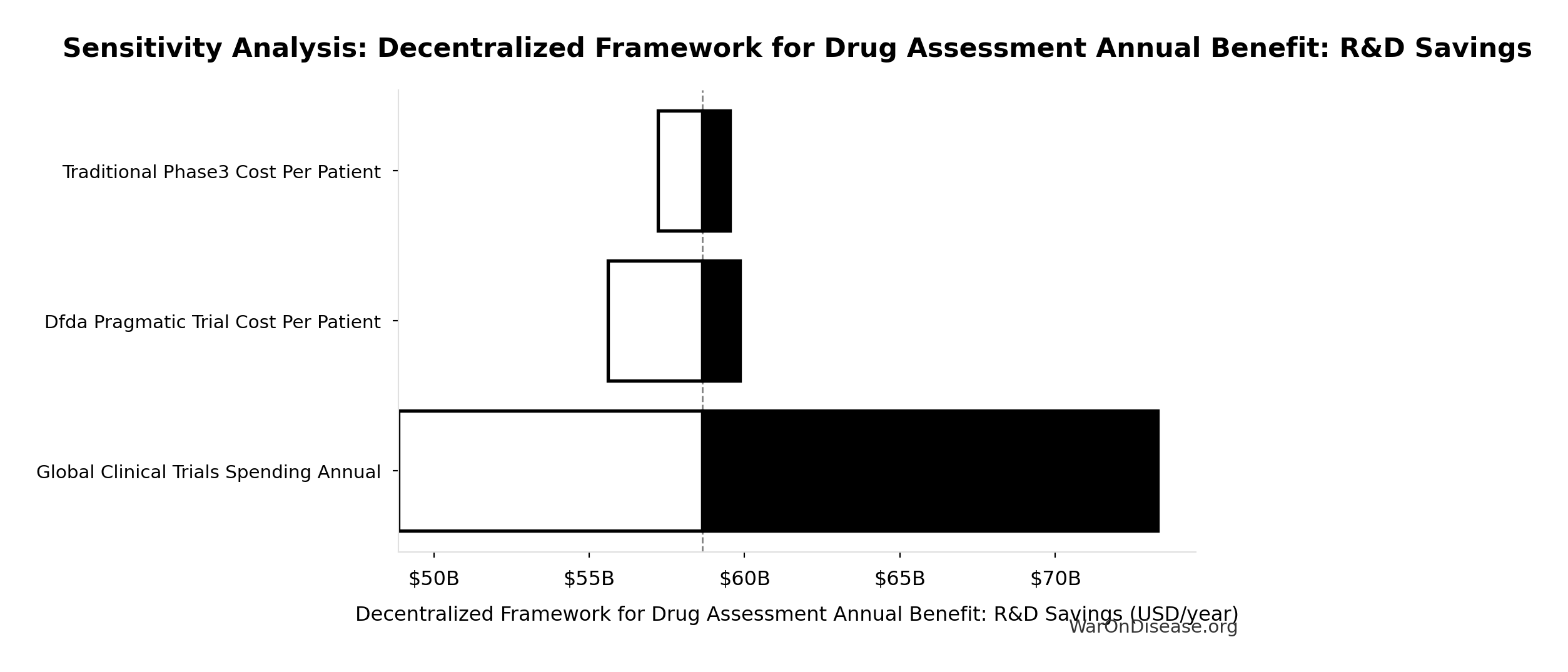
Sensitivity Indices for Decentralized Framework for Drug Assessment Annual Benefit: R&D Savings
Regression-based sensitivity showing which inputs explain the most variance in the output.
| Input Parameter | Sensitivity Coefficient | Interpretation |
|---|---|---|
| Global Clinical Trials Spending Annual | 1.0205 | Strong driver |
| dFDA Trial Cost Reduction % | 0.0244 | Minimal effect |
Interpretation: Standardized coefficients show the change in output (in SD units) per 1 SD change in input. Values near ±1 indicate strong influence; values exceeding ±1 may occur with correlated inputs.
Monte Carlo Distribution
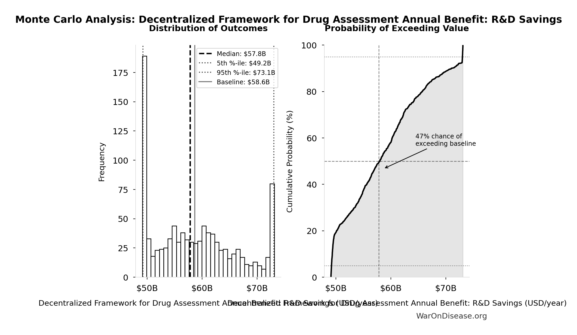
Simulation Results Summary: Decentralized Framework for Drug Assessment Annual Benefit: R&D Savings
| Statistic | Value |
|---|---|
| Baseline (deterministic) | $58.6B |
| Mean (expected value) | $58.8B |
| Median (50th percentile) | $57.8B |
| Standard Deviation | $7.66B |
| 90% Confidence Interval | [$49.2B, $73.1B] |
The histogram shows the distribution of Decentralized Framework for Drug Assessment Annual Benefit: R&D Savings across 10,000 Monte Carlo simulations. The CDF (right) shows the probability of the outcome exceeding any given value, which is useful for risk assessment.
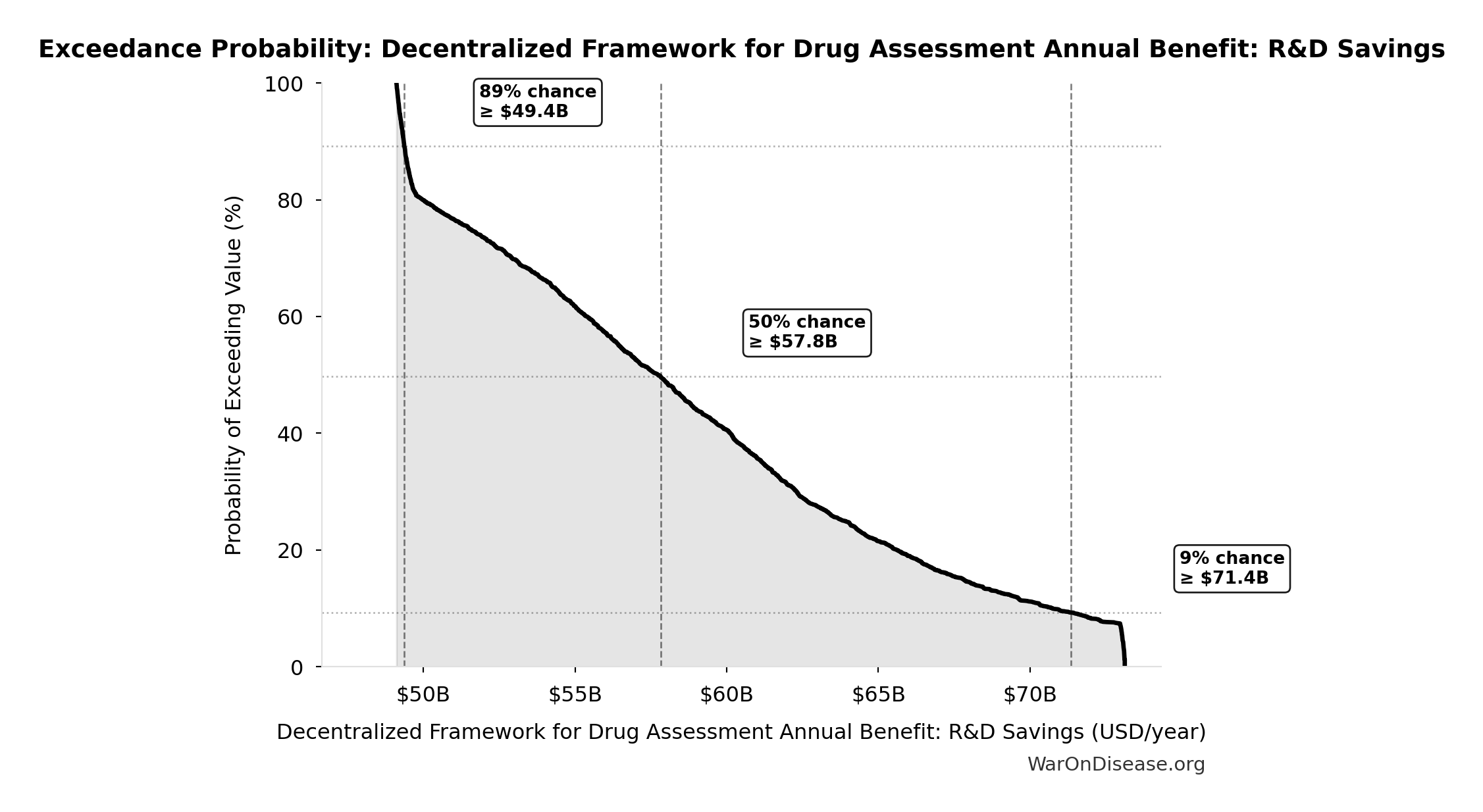
Exceedance Probability
This exceedance probability chart shows the likelihood that Decentralized Framework for Drug Assessment Annual Benefit: R&D Savings will exceed any given threshold. Higher curves indicate more favorable outcomes with greater certainty.
dFDA Trial Cost Reduction Percentage: 97.7%
Trial cost reduction percentage: (traditional - dFDA) / traditional = ($41K - $1.2K) / $41K = 97%
Inputs:
- dFDA Pragmatic Trial Cost per Patient 📊: $929 (95% CI: $97 - $3K)
- Phase 3 Cost per Patient 📊: $41K (95% CI: $20K - $120K)
\[ \begin{gathered} Reduce_{pct} \\ = 1 - \frac{Cost_{pragmatic,pt}}{Cost_{P3,pt}} \\ = 1 - \frac{\$929}{\$41K} \\ = 97.7\% \end{gathered} \]
✓ High confidence
Sensitivity Analysis
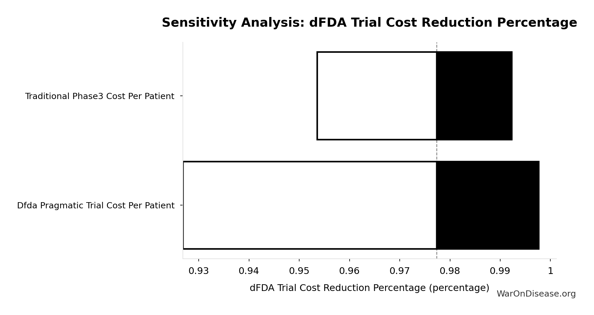
Sensitivity Indices for dFDA Trial Cost Reduction Percentage
Regression-based sensitivity showing which inputs explain the most variance in the output.
| Input Parameter | Sensitivity Coefficient | Interpretation |
|---|---|---|
| dFDA Pragmatic Trial Cost Per Patient | -6.4207 | Strong driver |
| Traditional Phase3 Cost Per Patient | 5.6539 | Strong driver |
Interpretation: Standardized coefficients show the change in output (in SD units) per 1 SD change in input. Values near ±1 indicate strong influence; values exceeding ±1 may occur with correlated inputs.
Monte Carlo Distribution
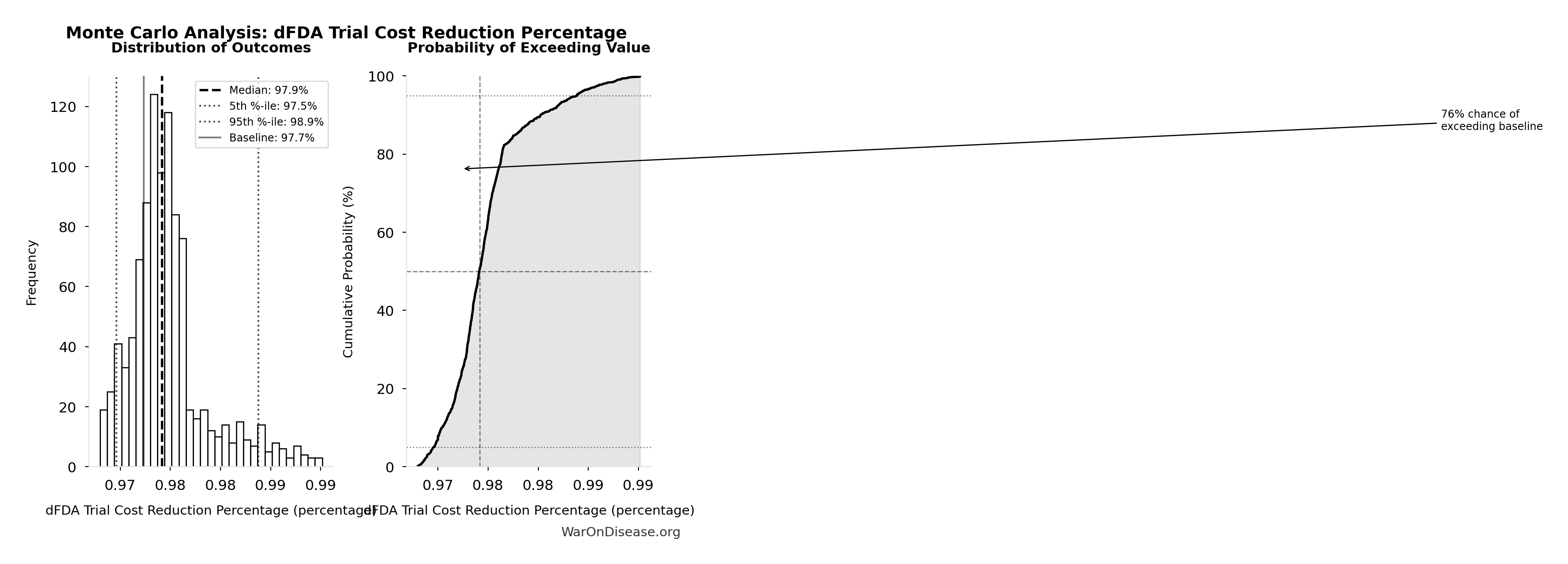
Simulation Results Summary: dFDA Trial Cost Reduction Percentage
| Statistic | Value |
|---|---|
| Baseline (deterministic) | 97.7% |
| Mean (expected value) | 98% |
| Median (50th percentile) | 97.9% |
| Standard Deviation | 0.401% |
| 90% Confidence Interval | [97.5%, 98.9%] |
The histogram shows the distribution of dFDA Trial Cost Reduction Percentage across 10,000 Monte Carlo simulations. The CDF (right) shows the probability of the outcome exceeding any given value, which is useful for risk assessment.
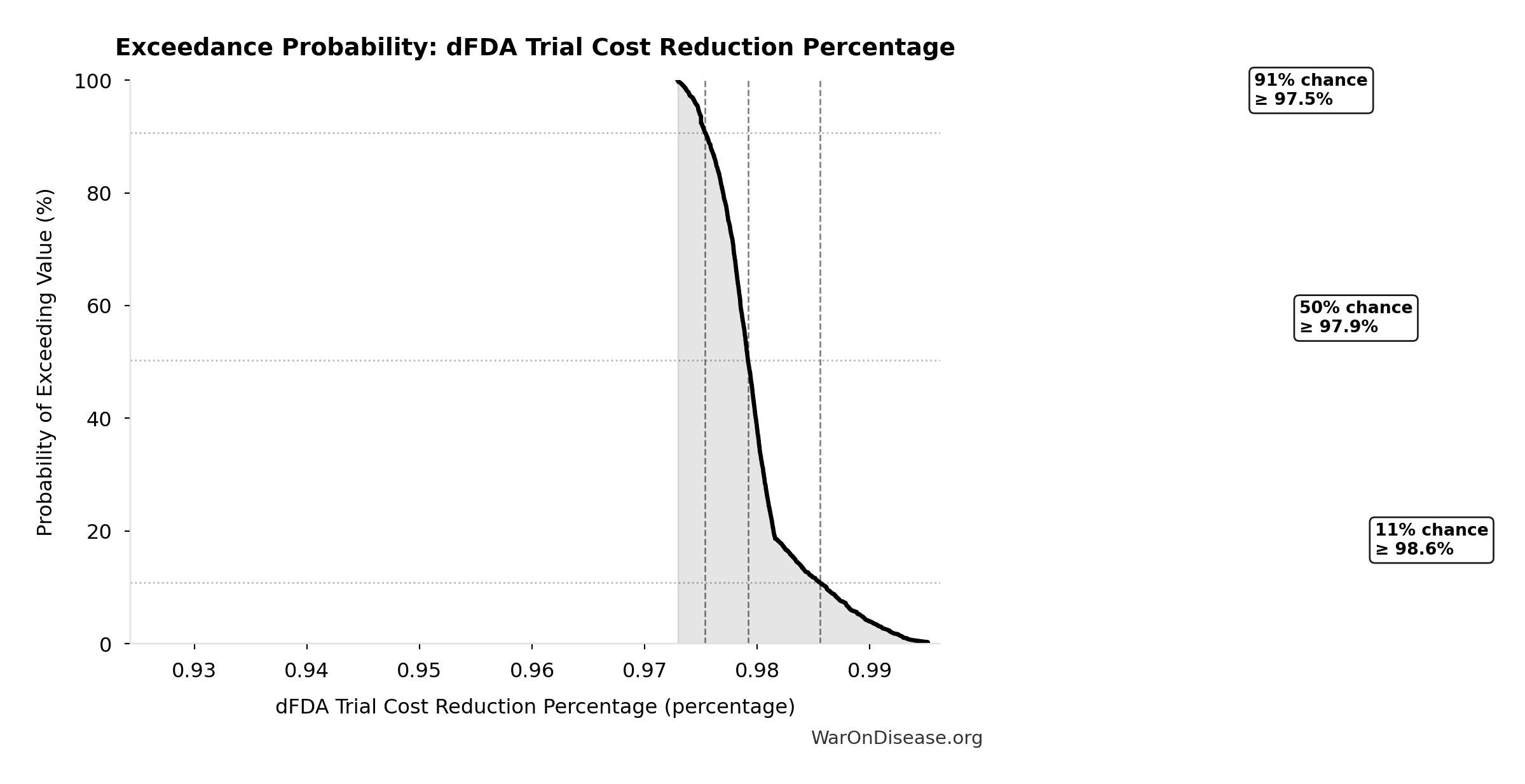
Exceedance Probability
This exceedance probability chart shows the likelihood that dFDA Trial Cost Reduction Percentage will exceed any given threshold. Higher curves indicate more favorable outcomes with greater certainty.
Total Annual Cost of War Worldwide: $11.4T
Total annual cost of war worldwide (direct + indirect costs)
Inputs:
- Total Annual Direct War Costs 🔢: $7.66T
- Total Annual Indirect War Costs 🔢: $3.70T
\[ \begin{gathered} Cost_{war,total} \\ = Cost_{war,direct} + Cost_{war,indirect} \\ = \$7.66T + \$3.7T \\ = \$11.4T \\[0.5em] \text{where } Cost_{war,direct} \\ = Loss_{life,conflict} + Damage_{infra,total} \\ + Disruption_{trade} + Spending_{mil} \\ = \$2.45T + \$1.88T + \$616B + \$2.72T \\ = \$7.66T \\[0.5em] \text{where } Loss_{life,conflict} \\ = Cost_{combat,human} + Cost_{state,human} \\ + Cost_{terror,human} \\ = \$2.34T + \$27B + \$83B \\ = \$2.45T \\[0.5em] \text{where } Cost_{combat,human} \\ = Deaths_{combat} \times VSL \\ = 234{,}000 \times \$10M \\ = \$2.34T \\[0.5em] \text{where } Cost_{state,human} \\ = Deaths_{state} \times VSL \\ = 2{,}700 \times \$10M \\ = \$27B \\[0.5em] \text{where } Cost_{terror,human} \\ = Deaths_{terror} \times VSL \\ = 8{,}300 \times \$10M \\ = \$83B \\[0.5em] \text{where } Damage_{infra,total} \\ = Damage_{comms} + Damage_{edu} + Damage_{energy} \\ + Damage_{health} + Damage_{transport} \\ + Damage_{water} \\ = \$298B + \$234B + \$422B + \$166B + \$487B + \$268B \\ = \$1.88T \\[0.5em] \text{where } Disruption_{trade} \\ = Disruption_{currency} + Disruption_{energy} \\ + Disruption_{shipping} + Disruption_{supply} \\ = \$57.4B + \$125B + \$247B + \$187B \\ = \$616B \\[0.5em] \text{where } Cost_{war,indirect} \\ = Damage_{env} + Loss_{growth,mil} \\ + Loss_{capital,conflict} + Cost_{psych} \\ + Cost_{refugee} + Cost_{vet} \\ = \$100B + \$2.72T + \$300B + \$232B + \$150B + \$200B \\ = \$3.7T \end{gathered} \]
✓ High confidence
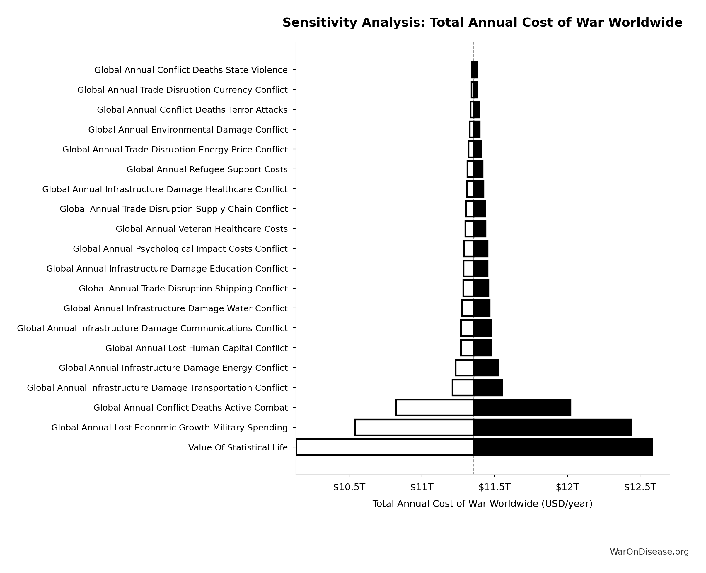
Sensitivity Analysis
Sensitivity Indices for Total Annual Cost of War Worldwide
Regression-based sensitivity showing which inputs explain the most variance in the output.
| Input Parameter | Sensitivity Coefficient | Interpretation |
|---|---|---|
| Global Annual War Direct Costs Total | 0.6553 | Strong driver |
| Global Annual War Indirect Costs Total | 0.4150 | Moderate driver |
Interpretation: Standardized coefficients show the change in output (in SD units) per 1 SD change in input. Values near ±1 indicate strong influence; values exceeding ±1 may occur with correlated inputs.
Monte Carlo Distribution
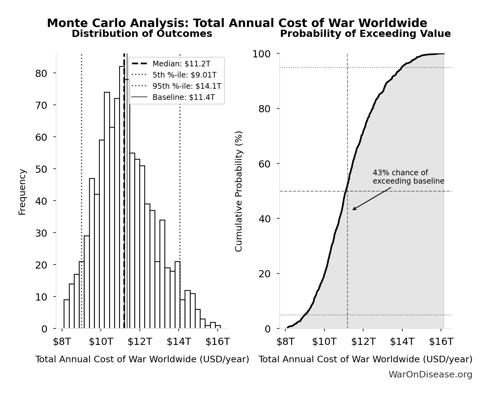
Simulation Results Summary: Total Annual Cost of War Worldwide
| Statistic | Value |
|---|---|
| Baseline (deterministic) | $11.4T |
| Mean (expected value) | $11.3T |
| Median (50th percentile) | $11.2T |
| Standard Deviation | $1.51T |
| 90% Confidence Interval | [$9.01T, $14.1T] |
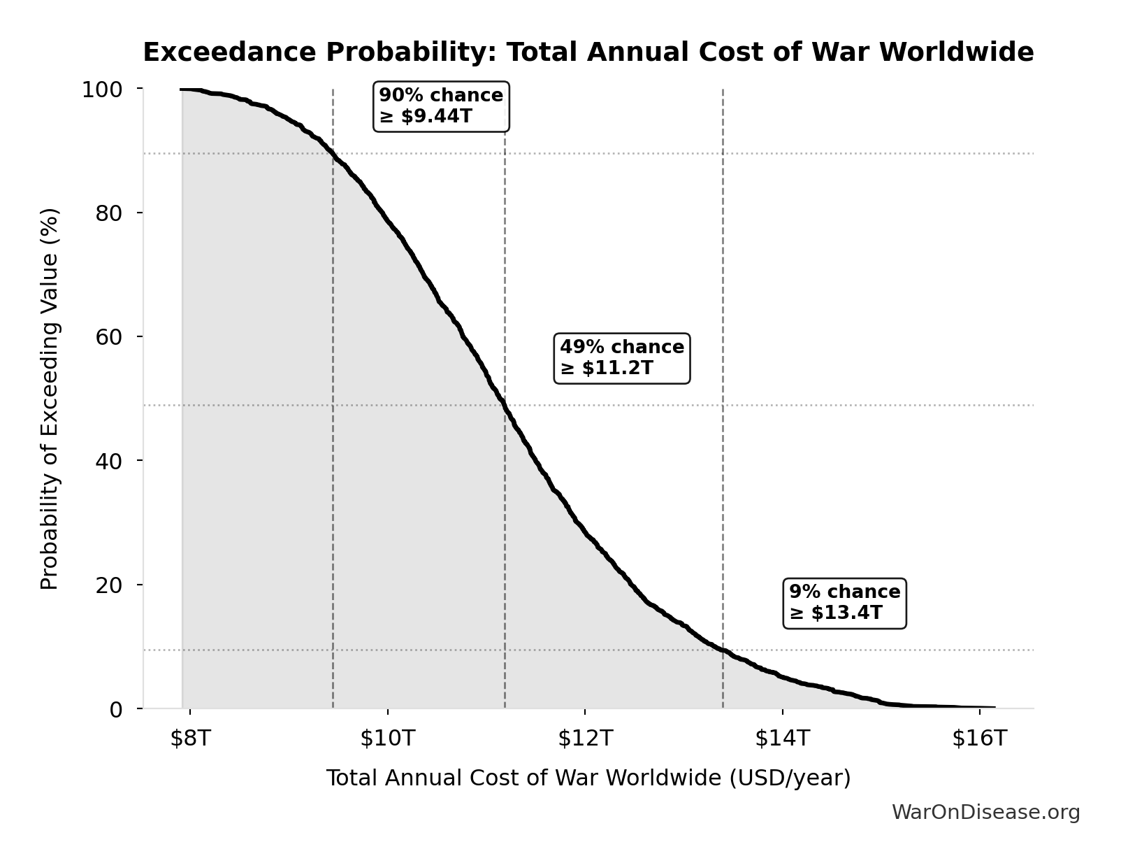
The histogram shows the distribution of Total Annual Cost of War Worldwide across 10,000 Monte Carlo simulations. The CDF (right) shows the probability of the outcome exceeding any given value, which is useful for risk assessment.
Exceedance Probability
This exceedance probability chart shows the likelihood that Total Annual Cost of War Worldwide will exceed any given threshold. Higher curves indicate more favorable outcomes with greater certainty.
Annual Cost of Combat Deaths: $2.34T
Annual cost of combat deaths (deaths × VSL)
Inputs:
- Annual Deaths from Active Combat Worldwide 📊: 234k deaths/year (95% CI: 180k deaths/year - 300k deaths/year)
- Value of Statistical Life 📊: $10M (95% CI: $5M - $15M)
\[ \begin{gathered} Cost_{combat,human} \\ = Deaths_{combat} \times VSL \\ = 234{,}000 \times \$10M \\ = \$2.34T \end{gathered} \]
✓ High confidence
Sensitivity Analysis
Sensitivity Indices for Annual Cost of Combat Deaths
Regression-based sensitivity showing which inputs explain the most variance in the output.
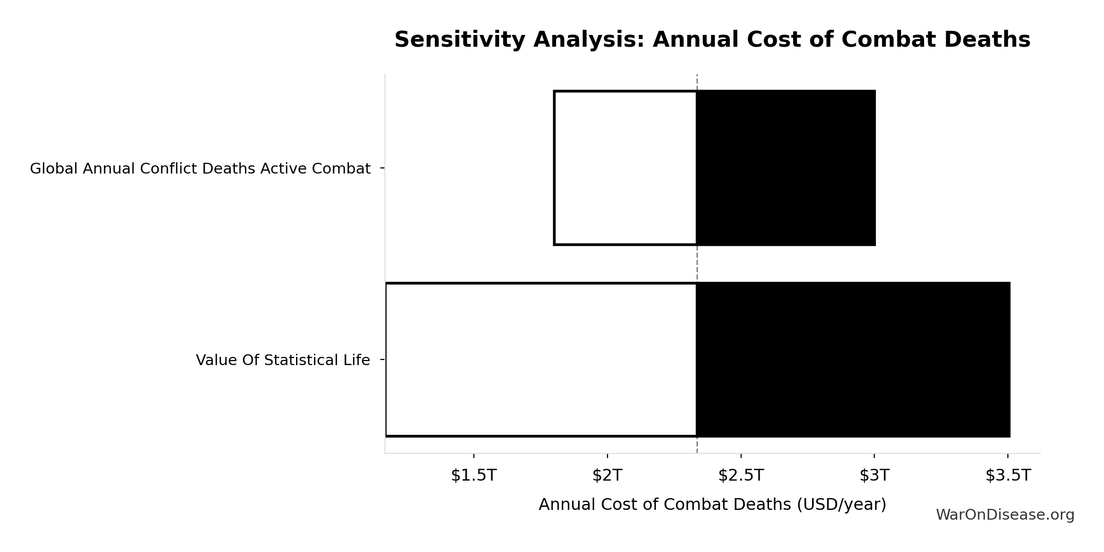
| Input Parameter | Sensitivity Coefficient | Interpretation |
|---|---|---|
| Value Of Statistical Life | 0.9096 | Strong driver |
| Global Annual Conflict Deaths Active Combat | 0.4115 | Moderate driver |
Interpretation: Standardized coefficients show the change in output (in SD units) per 1 SD change in input. Values near ±1 indicate strong influence; values exceeding ±1 may occur with correlated inputs.
Monte Carlo Distribution
Simulation Results Summary: Annual Cost of Combat Deaths
| Statistic | Value |
|---|---|
| Baseline (deterministic) | $2.34T |
| Mean (expected value) | $2.31T |
| Median (50th percentile) | $2.24T |
| Standard Deviation | $703B |
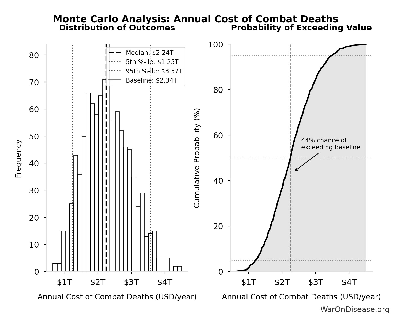
| 90% Confidence Interval | [$1.25T, $3.57T] |
The histogram shows the distribution of Annual Cost of Combat Deaths across 10,000 Monte Carlo simulations. The CDF (right) shows the probability of the outcome exceeding any given value, which is useful for risk assessment.
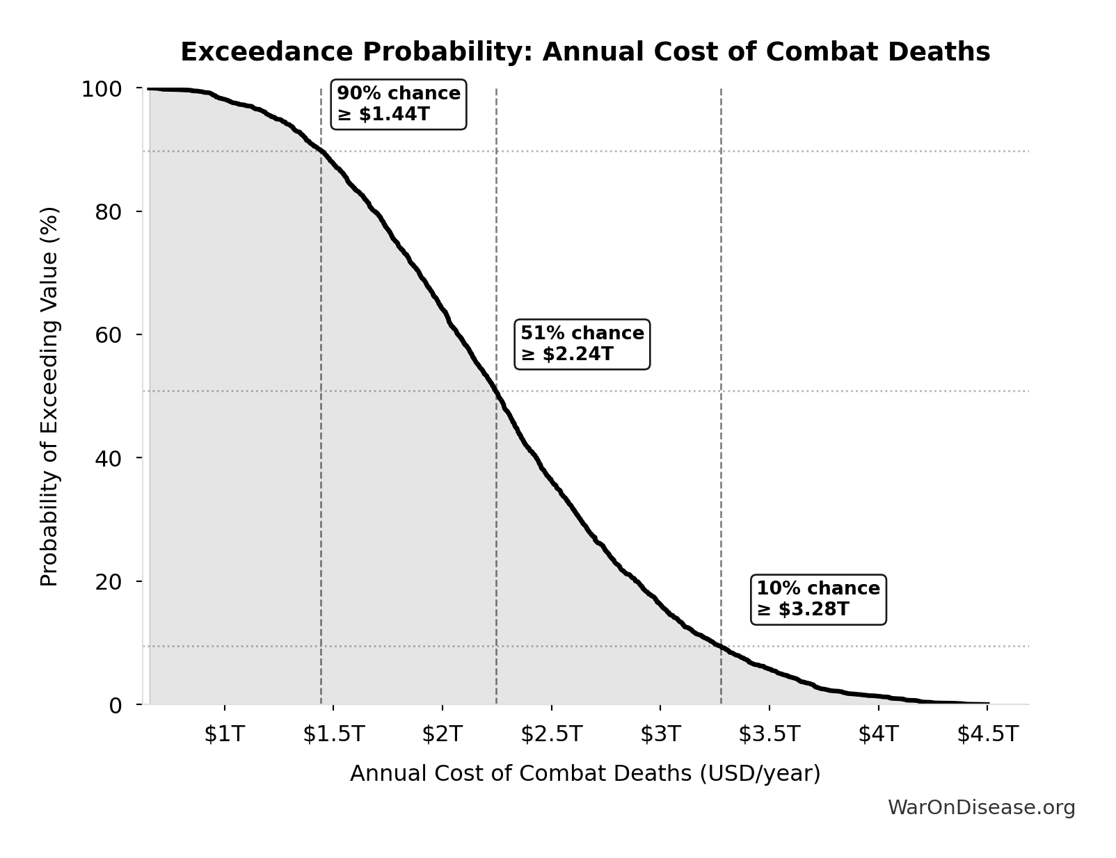
Exceedance Probability
This exceedance probability chart shows the likelihood that Annual Cost of Combat Deaths will exceed any given threshold. Higher curves indicate more favorable outcomes with greater certainty.
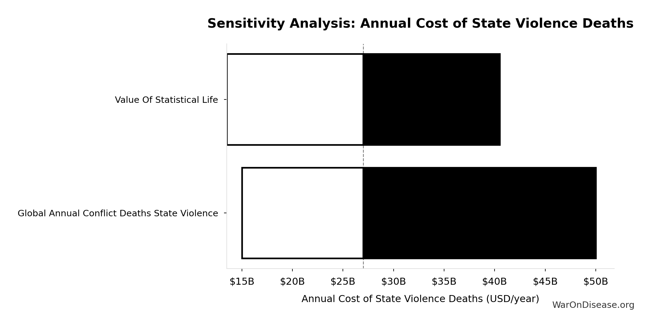
Annual Cost of State Violence Deaths: $27B
Annual cost of state violence deaths (deaths × VSL)
Inputs:
- Annual Deaths from State Violence 📊: 2.70k deaths/year (95% CI: 1.50k deaths/year - 5.00k deaths/year)
- Value of Statistical Life 📊: $10M (95% CI: $5M - $15M)
\[ \begin{gathered} Cost_{state,human} \\ = Deaths_{state} \times VSL \\ = 2{,}700 \times \$10M \\ = \$27B \end{gathered} \]
✓ High confidence
Sensitivity Analysis
Sensitivity Indices for Annual Cost of State Violence Deaths
Regression-based sensitivity showing which inputs explain the most variance in the output.
| Input Parameter | Sensitivity Coefficient | Interpretation |
|---|---|---|
| Global Annual Conflict Deaths State Violence | 0.7358 | Strong driver |
| Value Of Statistical Life | 0.6553 | Strong driver |
Interpretation: Standardized coefficients show the change in output (in SD units) per 1 SD change in input. Values near ±1 indicate strong influence; values exceeding ±1 may occur with correlated inputs.
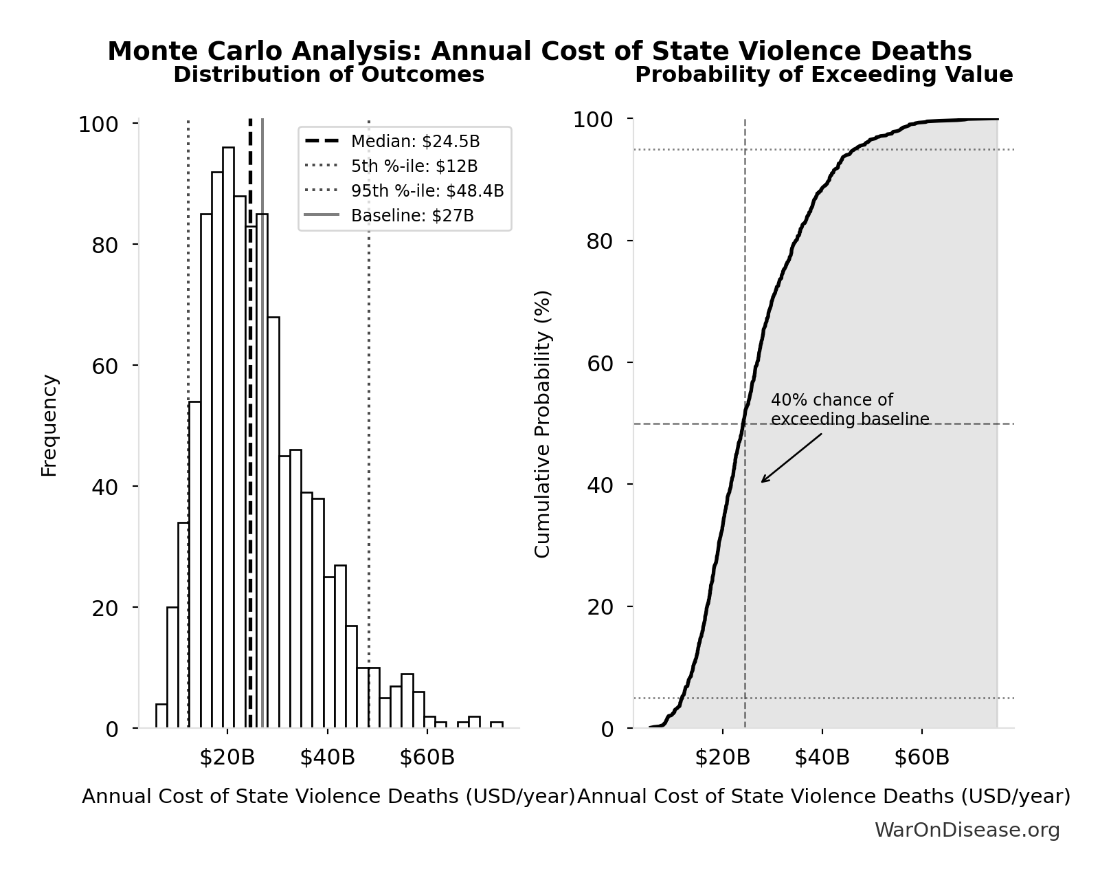
Monte Carlo Distribution
Simulation Results Summary: Annual Cost of State Violence Deaths
| Statistic | Value |
|---|---|
| Baseline (deterministic) | $27B |
| Mean (expected value) | $26.6B |
| Median (50th percentile) | $24.5B |
| Standard Deviation | $11.3B |
| 90% Confidence Interval | [$12B, $48.4B] |
The histogram shows the distribution of Annual Cost of State Violence Deaths across 10,000 Monte Carlo simulations. The CDF (right) shows the probability of the outcome exceeding any given value, which is useful for risk assessment.
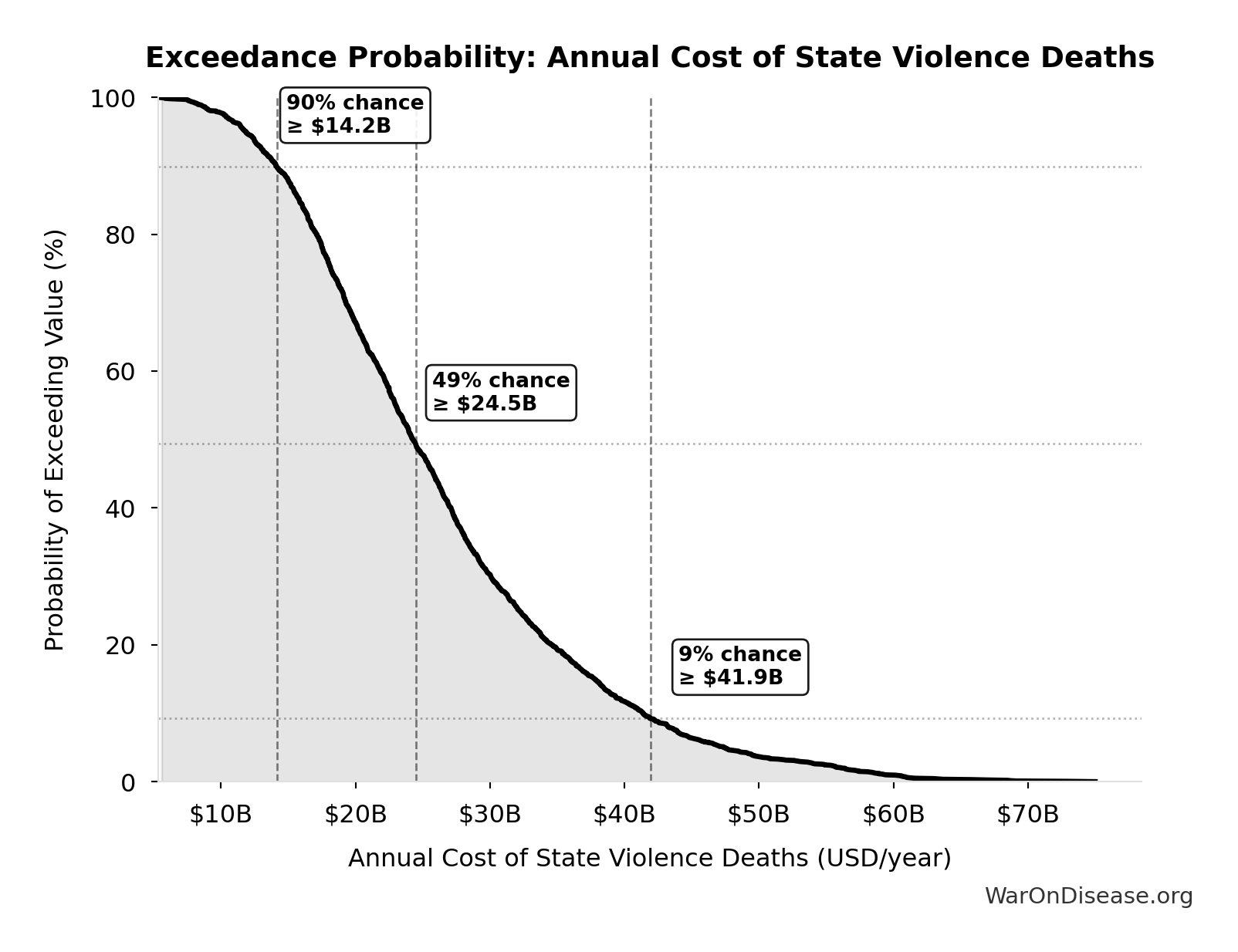
Exceedance Probability
This exceedance probability chart shows the likelihood that Annual Cost of State Violence Deaths will exceed any given threshold. Higher curves indicate more favorable outcomes with greater certainty.
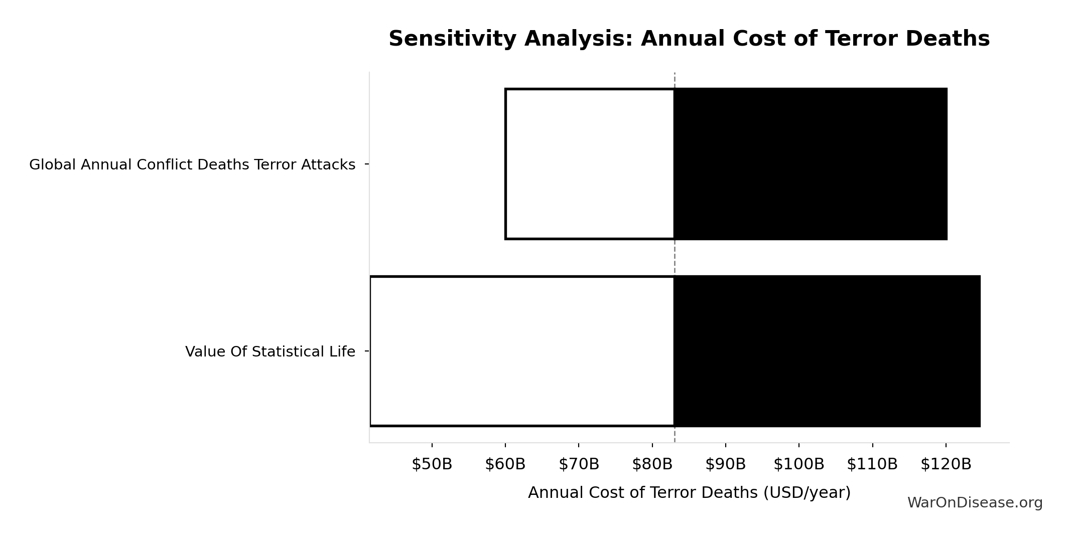
Annual Cost of Terror Deaths: $83B
Annual cost of terror deaths (deaths × VSL)
Inputs:
- Annual Deaths from Terror Attacks Globally 📊: 8.30k deaths/year (95% CI: 6.00k deaths/year - 12.0k deaths/year)
- Value of Statistical Life 📊: $10M (95% CI: $5M - $15M)
\[ \begin{gathered} Cost_{terror,human} \\ = Deaths_{terror} \times VSL \\ = 8{,}300 \times \$10M \\ = \$83B \end{gathered} \]
✓ High confidence
Sensitivity Analysis
Sensitivity Indices for Annual Cost of Terror Deaths
Regression-based sensitivity showing which inputs explain the most variance in the output.
| Input Parameter | Sensitivity Coefficient | Interpretation |
|---|---|---|
| Value Of Statistical Life | 0.8410 | Strong driver |
| Global Annual Conflict Deaths Terror Attacks | 0.5319 | Strong driver |
Interpretation: Standardized coefficients show the change in output (in SD units) per 1 SD change in input. Values near ±1 indicate strong influence; values exceeding ±1 may occur with correlated inputs.
Monte Carlo Distribution
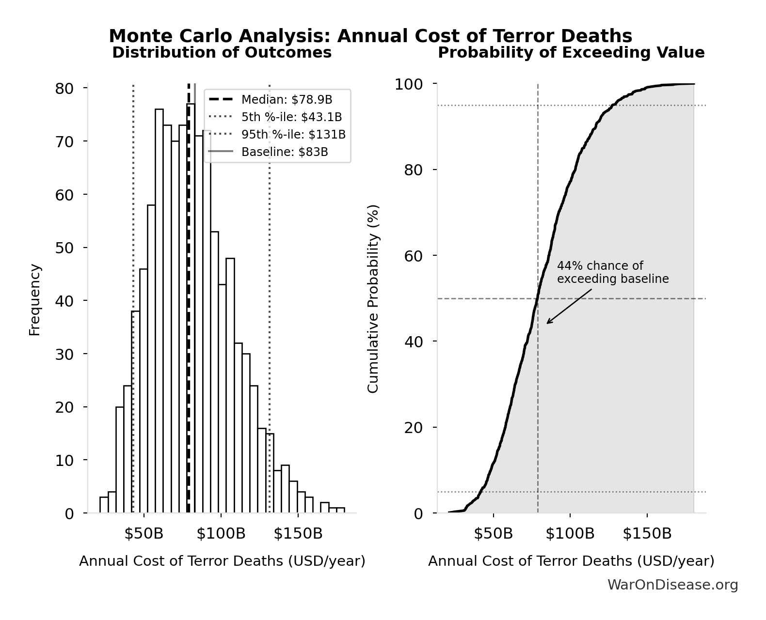
Simulation Results Summary: Annual Cost of Terror Deaths
| Statistic | Value |
|---|---|
| Baseline (deterministic) | $83B |
| Mean (expected value) | $82.1B |
| Median (50th percentile) | $78.9B |
| Standard Deviation | $27B |
| 90% Confidence Interval | [$43.1B, $131B] |
The histogram shows the distribution of Annual Cost of Terror Deaths across 10,000 Monte Carlo simulations. The CDF (right) shows the probability of the outcome exceeding any given value, which is useful for risk assessment.
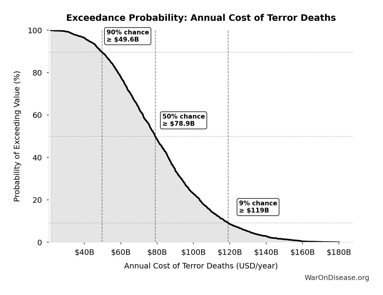
Exceedance Probability
This exceedance probability chart shows the likelihood that Annual Cost of Terror Deaths will exceed any given threshold. Higher curves indicate more favorable outcomes with greater certainty.
Total Annual Human Life Losses from Conflict: $2.45T
Total annual human life losses from conflict (sum of combat, terror, state violence)
Inputs:
- Annual Cost of Combat Deaths 🔢: $2.34T
- Annual Cost of State Violence Deaths 🔢: $27B
- Annual Cost of Terror Deaths 🔢: $83B
\[ \begin{gathered} Loss_{life,conflict} \\ = Cost_{combat,human} + Cost_{state,human} \\ + Cost_{terror,human} \\ = \$2.34T + \$27B + \$83B \\ = \$2.45T \\[0.5em] \text{where } Cost_{combat,human} \\ = Deaths_{combat} \times VSL \\ = 234{,}000 \times \$10M \\ = \$2.34T \\[0.5em] \text{where } Cost_{state,human} \\ = Deaths_{state} \times VSL \\ = 2{,}700 \times \$10M \\ = \$27B \\[0.5em] \text{where } Cost_{terror,human} \\ = Deaths_{terror} \times VSL \\ = 8{,}300 \times \$10M \\ = \$83B \end{gathered} \]
✓ High confidence
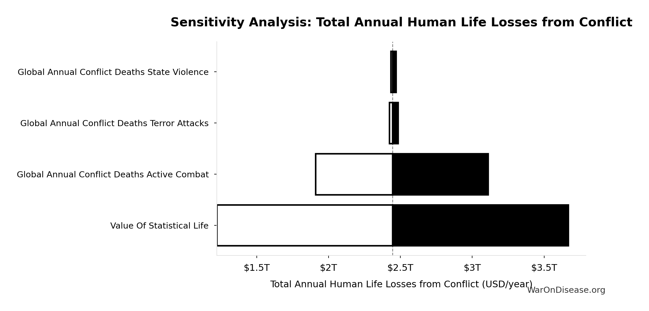
Sensitivity Analysis
Sensitivity Indices for Total Annual Human Life Losses from Conflict
Regression-based sensitivity showing which inputs explain the most variance in the output.
| Input Parameter | Sensitivity Coefficient | Interpretation |
|---|---|---|
| Global Annual Human Cost Active Combat | 0.9500 | Strong driver |
| Global Annual Human Cost Terror Attacks | 0.0365 | Minimal effect |
| Global Annual Human Cost State Violence | 0.0152 | Minimal effect |
Interpretation: Standardized coefficients show the change in output (in SD units) per 1 SD change in input. Values near ±1 indicate strong influence; values exceeding ±1 may occur with correlated inputs.
Monte Carlo Distribution
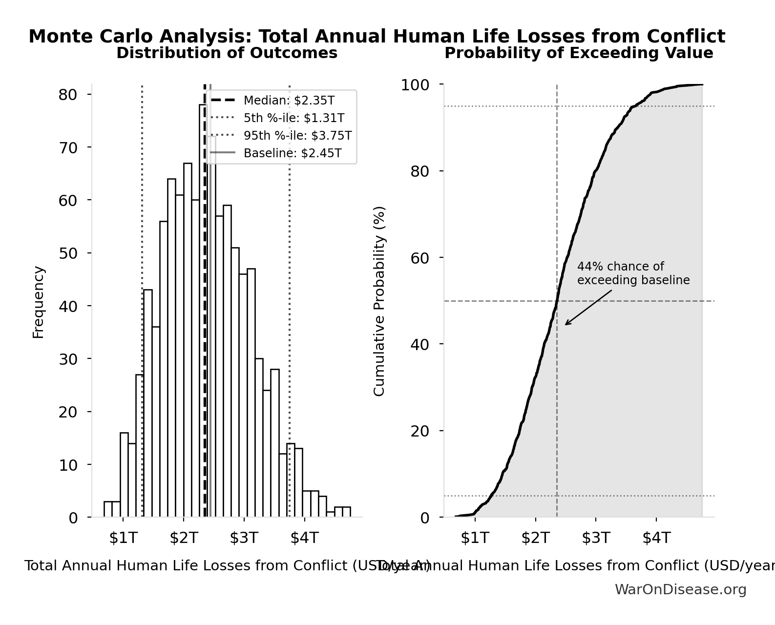
Simulation Results Summary: Total Annual Human Life Losses from Conflict
| Statistic | Value |
|---|---|
| Baseline (deterministic) | $2.45T |
| Mean (expected value) | $2.42T |
| Median (50th percentile) | $2.35T |
| Standard Deviation | $740B |
| 90% Confidence Interval | [$1.31T, $3.75T] |
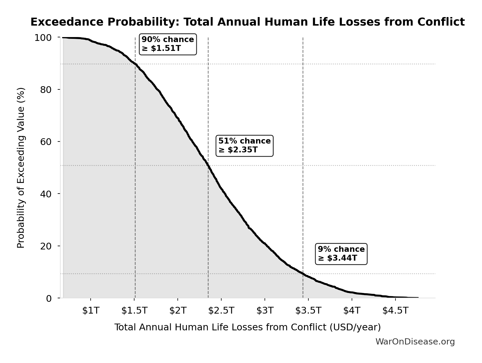
The histogram shows the distribution of Total Annual Human Life Losses from Conflict across 10,000 Monte Carlo simulations. The CDF (right) shows the probability of the outcome exceeding any given value, which is useful for risk assessment.
Exceedance Probability
This exceedance probability chart shows the likelihood that Total Annual Human Life Losses from Conflict will exceed any given threshold. Higher curves indicate more favorable outcomes with greater certainty.
Total Annual Infrastructure Destruction: $1.88T
Total annual infrastructure destruction (sum of transportation, energy, communications, water, education, healthcare)
Inputs:
- Annual Infrastructure Damage to Communications from Conflict 📊: $298B (95% CI: $209B - $418B)
- Annual Infrastructure Damage to Education Facilities from Conflict 📊: $234B (95% CI: $164B - $328B)
- Annual Infrastructure Damage to Energy Systems from Conflict 📊: $422B (95% CI: $295B - $590B)
- Annual Infrastructure Damage to Healthcare Facilities from Conflict 📊: $166B (95% CI: $116B - $232B)
- Annual Infrastructure Damage to Transportation from Conflict 📊: $487B (95% CI: $340B - $680B)
- Annual Infrastructure Damage to Water Systems from Conflict 📊: $268B (95% CI: $187B - $375B)
\[ \begin{gathered} Damage_{infra,total} \\ = Damage_{comms} + Damage_{edu} + Damage_{energy} \\ + Damage_{health} + Damage_{transport} + Damage_{water} \\ = \$298B + \$234B + \$422B + \$166B + \$487B + \$268B \\ = \$1.88T \end{gathered} \]
✓ High confidence
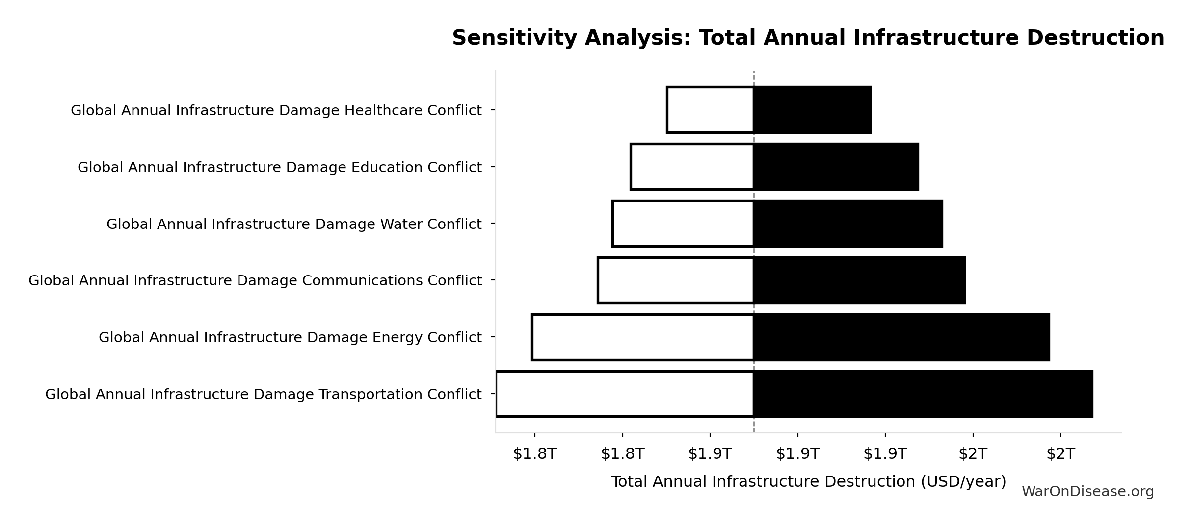
Sensitivity Analysis
Sensitivity Indices for Total Annual Infrastructure Destruction
Regression-based sensitivity showing which inputs explain the most variance in the output.
| Input Parameter | Sensitivity Coefficient | Interpretation |
|---|---|---|
| Global Annual Infrastructure Damage Transportation Conflict | 0.2591 | Weak driver |
| Global Annual Infrastructure Damage Energy Conflict | 0.2249 | Weak driver |
| Global Annual Infrastructure Damage Communications Conflict | 0.1593 | Weak driver |
| Global Annual Infrastructure Damage Water Conflict | 0.1433 | Weak driver |
| Global Annual Infrastructure Damage Education Conflict | 0.1250 | Weak driver |
| Global Annual Infrastructure Damage Healthcare Conflict | 0.0884 | Minimal effect |
Interpretation: Standardized coefficients show the change in output (in SD units) per 1 SD change in input. Values near ±1 indicate strong influence; values exceeding ±1 may occur with correlated inputs.
Monte Carlo Distribution
Simulation Results Summary: Total Annual Infrastructure Destruction
| Statistic | Value |
|---|---|
| Baseline (deterministic) | $1.88T |
| Mean (expected value) | $1.87T |
| Median (50th percentile) | $1.84T |
| Standard Deviation | $319B |
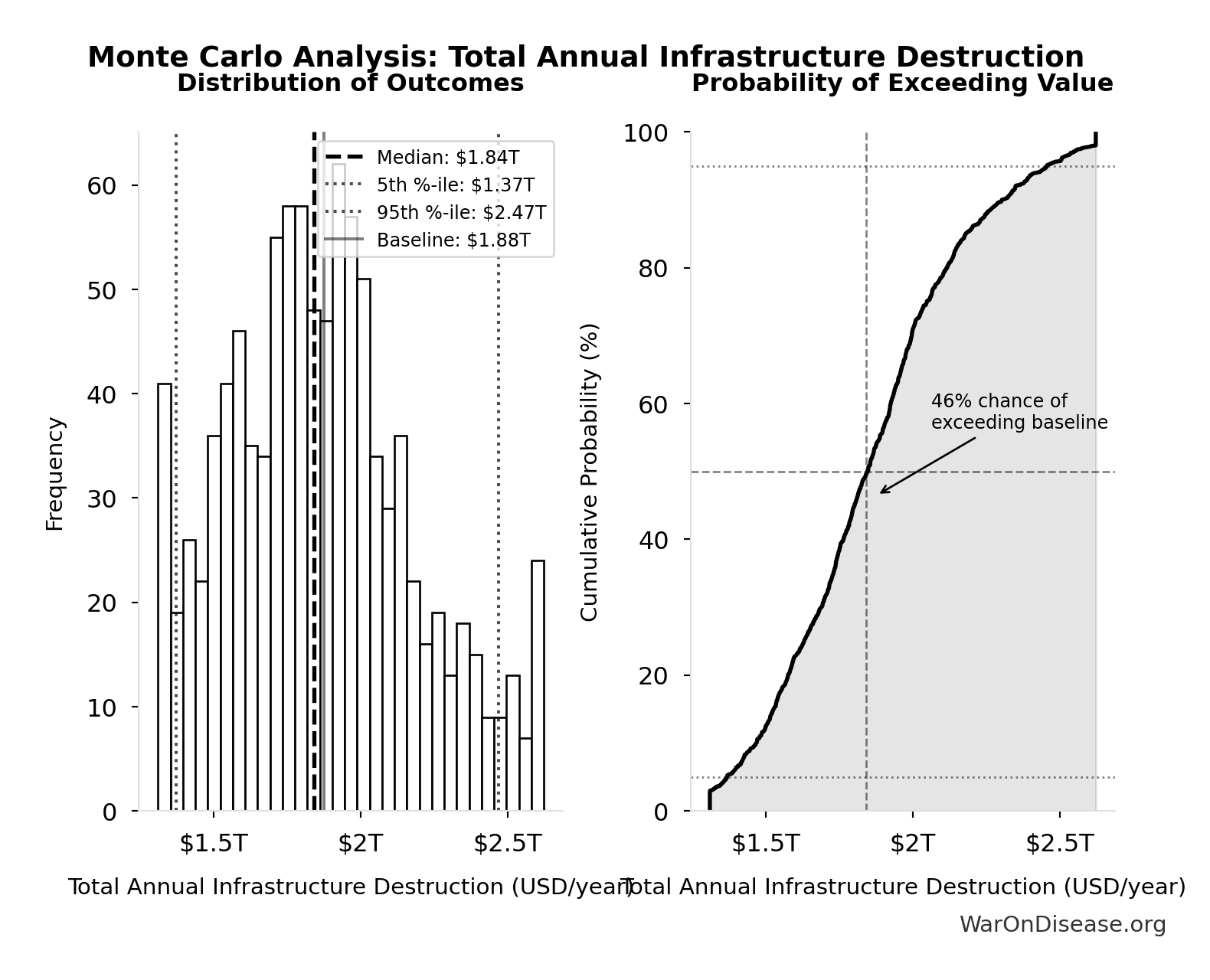
| 90% Confidence Interval | [$1.37T, $2.47T] |
The histogram shows the distribution of Total Annual Infrastructure Destruction across 10,000 Monte Carlo simulations. The CDF (right) shows the probability of the outcome exceeding any given value, which is useful for risk assessment.
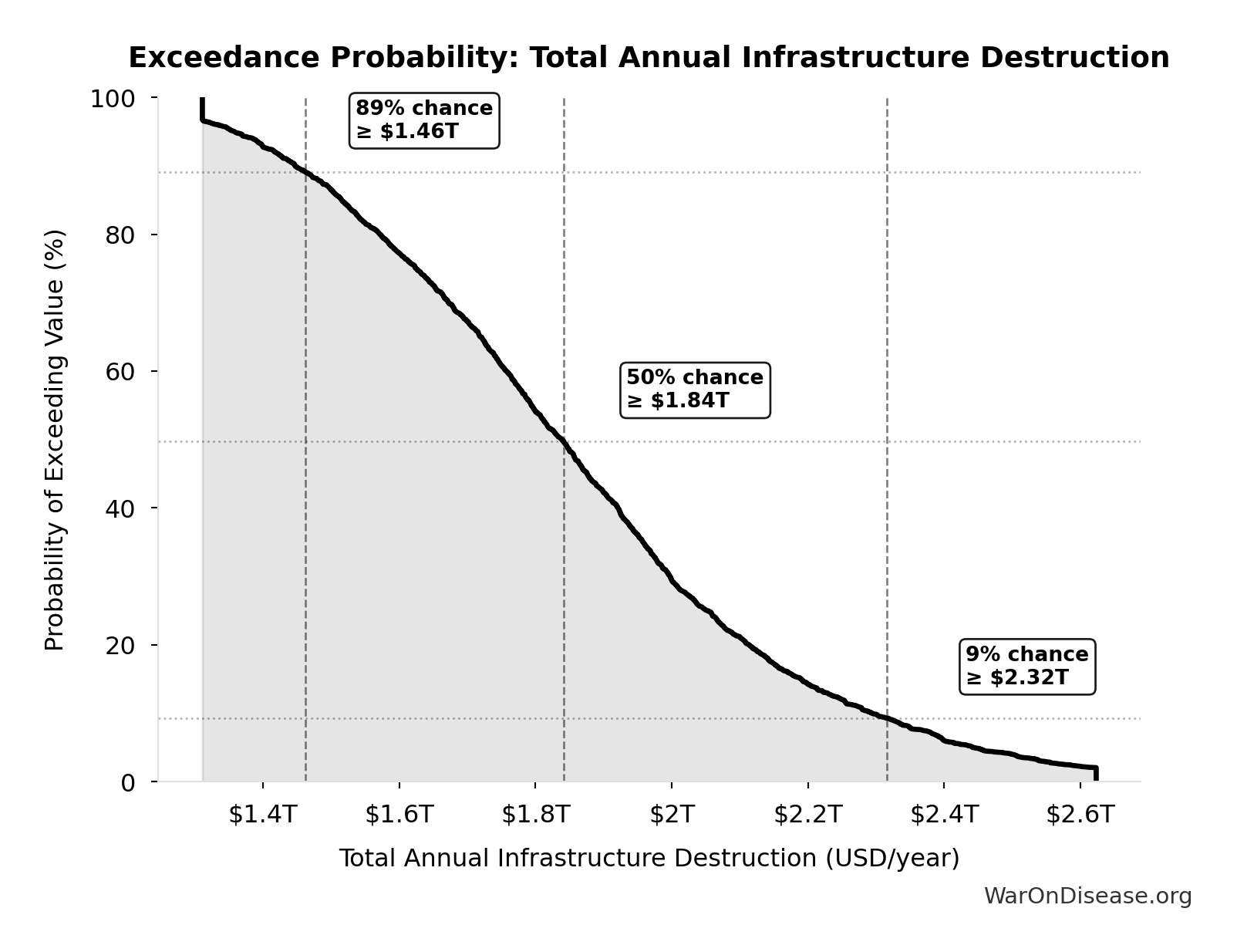
Exceedance Probability
This exceedance probability chart shows the likelihood that Total Annual Infrastructure Destruction will exceed any given threshold. Higher curves indicate more favorable outcomes with greater certainty.
Total Annual Trade Disruption: $616B
Total annual trade disruption (sum of shipping, supply chain, energy prices, currency instability)
Inputs:
- Annual Trade Disruption Costs from Currency Instability 📊: $57.4B (95% CI: $40B - $80B)
- Annual Trade Disruption Costs from Energy Price Volatility 📊: $125B (95% CI: $87B - $175B)
- Annual Trade Disruption Costs from Shipping Disruptions 📊: $247B (95% CI: $173B - $346B)
- Annual Trade Disruption Costs from Supply Chain Disruptions 📊: $187B (95% CI: $131B - $262B)
\[ \begin{gathered} Disruption_{trade} \\ = Disruption_{currency} + Disruption_{energy} \\ + Disruption_{shipping} + Disruption_{supply} \\ = \$57.4B + \$125B + \$247B + \$187B \\ = \$616B \end{gathered} \]
✓ High confidence
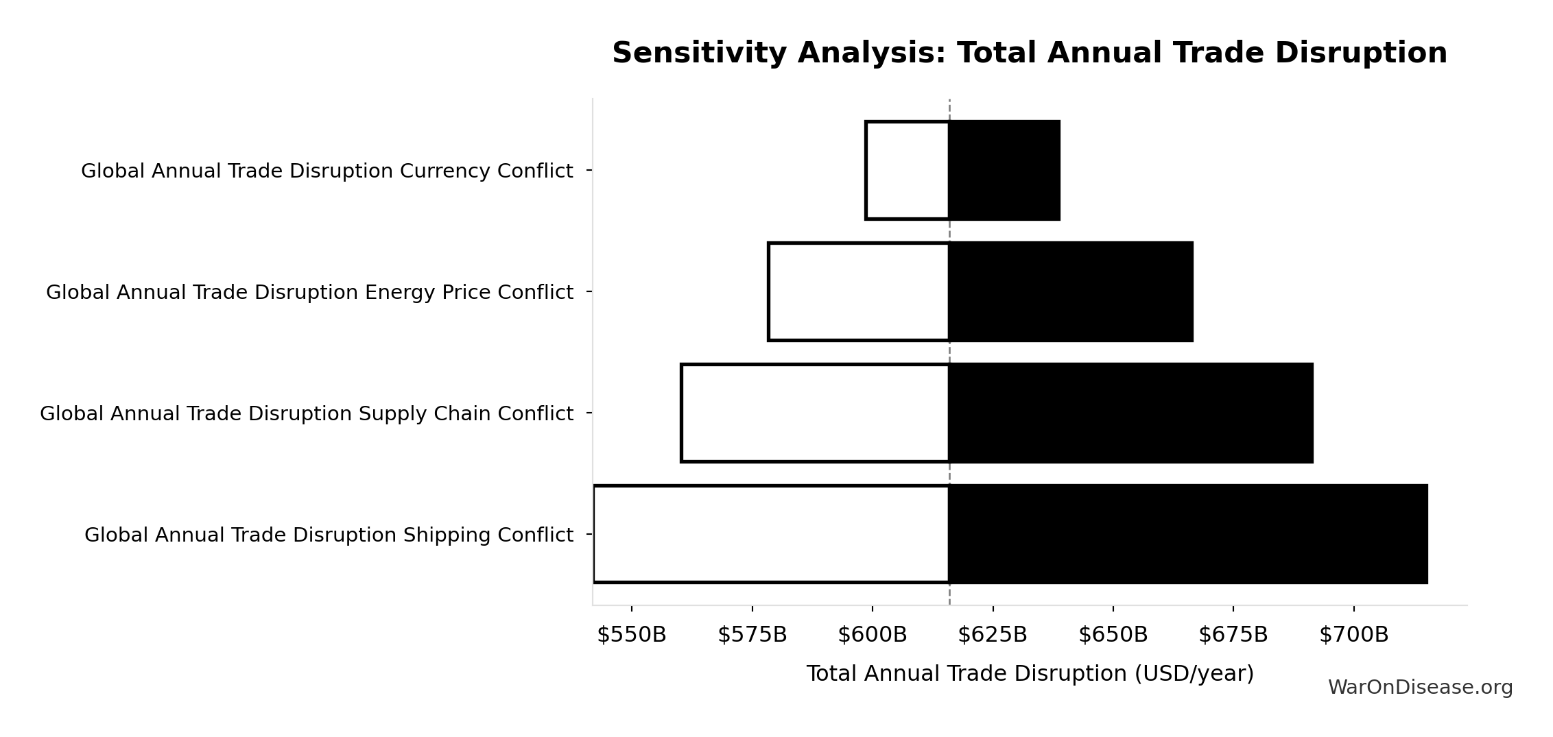
Sensitivity Analysis
Sensitivity Indices for Total Annual Trade Disruption
Regression-based sensitivity showing which inputs explain the most variance in the output.
| Input Parameter | Sensitivity Coefficient | Interpretation |
|---|---|---|
| Global Annual Trade Disruption Shipping Conflict | 0.4005 | Moderate driver |
| Global Annual Trade Disruption Supply Chain Conflict | 0.3033 | Moderate driver |
| Global Annual Trade Disruption Energy Price Conflict | 0.2037 | Weak driver |
| Global Annual Trade Disruption Currency Conflict | 0.0926 | Minimal effect |
Interpretation: Standardized coefficients show the change in output (in SD units) per 1 SD change in input. Values near ±1 indicate strong influence; values exceeding ±1 may occur with correlated inputs.
Monte Carlo Distribution
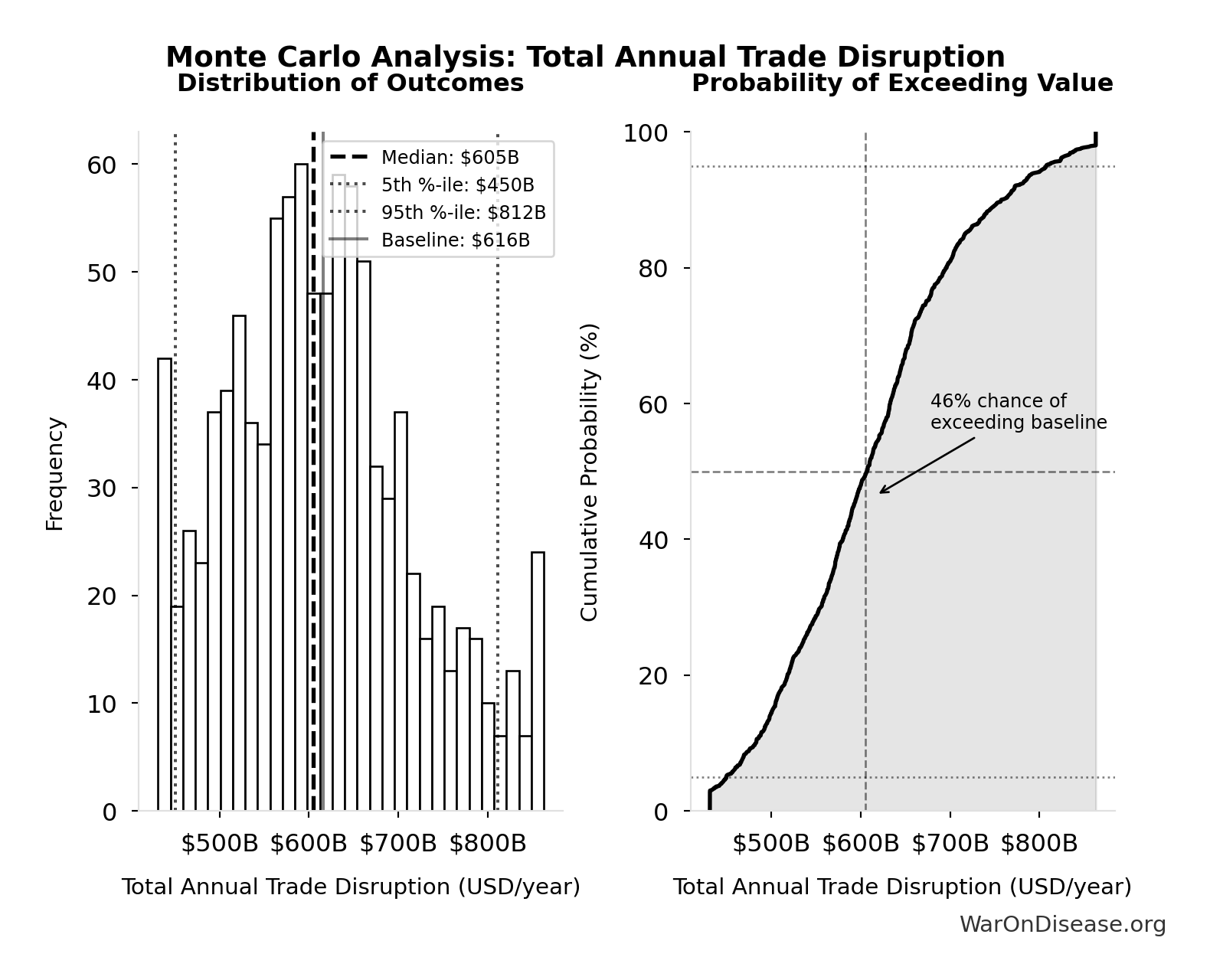
Simulation Results Summary: Total Annual Trade Disruption
| Statistic | Value |
|---|---|
| Baseline (deterministic) | $616B |
| Mean (expected value) | $614B |
| Median (50th percentile) | $605B |
| Standard Deviation | $105B |
| 90% Confidence Interval | [$450B, $812B] |
The histogram shows the distribution of Total Annual Trade Disruption across 10,000 Monte Carlo simulations. The CDF (right) shows the probability of the outcome exceeding any given value, which is useful for risk assessment.
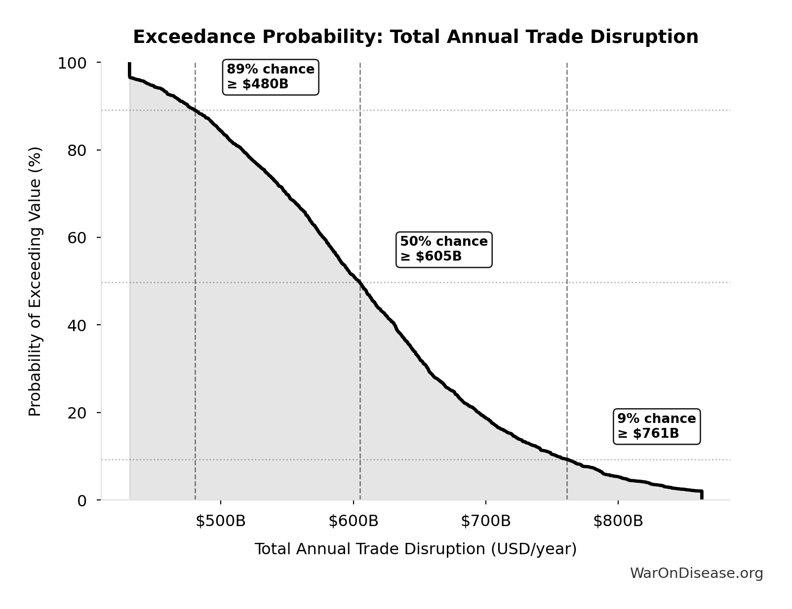
Exceedance Probability
This exceedance probability chart shows the likelihood that Total Annual Trade Disruption will exceed any given threshold. Higher curves indicate more favorable outcomes with greater certainty.
Total Annual Direct War Costs: $7.66T
Total annual direct war costs (military spending + infrastructure + human life + trade disruption)
Inputs:
- Total Annual Human Life Losses from Conflict 🔢: $2.45T
- Total Annual Infrastructure Destruction 🔢: $1.88T
- Total Annual Trade Disruption 🔢: $616B
- Global Military Spending in 2024 📊: $2.72T
\[ \begin{gathered} Cost_{war,direct} \\ = Loss_{life,conflict} + Damage_{infra,total} \\ + Disruption_{trade} + Spending_{mil} \\ = \$2.45T + \$1.88T + \$616B + \$2.72T \\ = \$7.66T \\[0.5em] \text{where } Loss_{life,conflict} \\ = Cost_{combat,human} + Cost_{state,human} \\ + Cost_{terror,human} \\ = \$2.34T + \$27B + \$83B \\ = \$2.45T \\[0.5em] \text{where } Cost_{combat,human} \\ = Deaths_{combat} \times VSL \\ = 234{,}000 \times \$10M \\ = \$2.34T \\[0.5em] \text{where } Cost_{state,human} \\ = Deaths_{state} \times VSL \\ = 2{,}700 \times \$10M \\ = \$27B \\[0.5em] \text{where } Cost_{terror,human} \\ = Deaths_{terror} \times VSL \\ = 8{,}300 \times \$10M \\ = \$83B \\[0.5em] \text{where } Damage_{infra,total} \\ = Damage_{comms} + Damage_{edu} + Damage_{energy} \\ + Damage_{health} + Damage_{transport} \\ + Damage_{water} \\ = \$298B + \$234B + \$422B + \$166B + \$487B + \$268B \\ = \$1.88T \\[0.5em] \text{where } Disruption_{trade} \\ = Disruption_{currency} + Disruption_{energy} \\ + Disruption_{shipping} + Disruption_{supply} \\ = \$57.4B + \$125B + \$247B + \$187B \\ = \$616B \end{gathered} \]
✓ High confidence
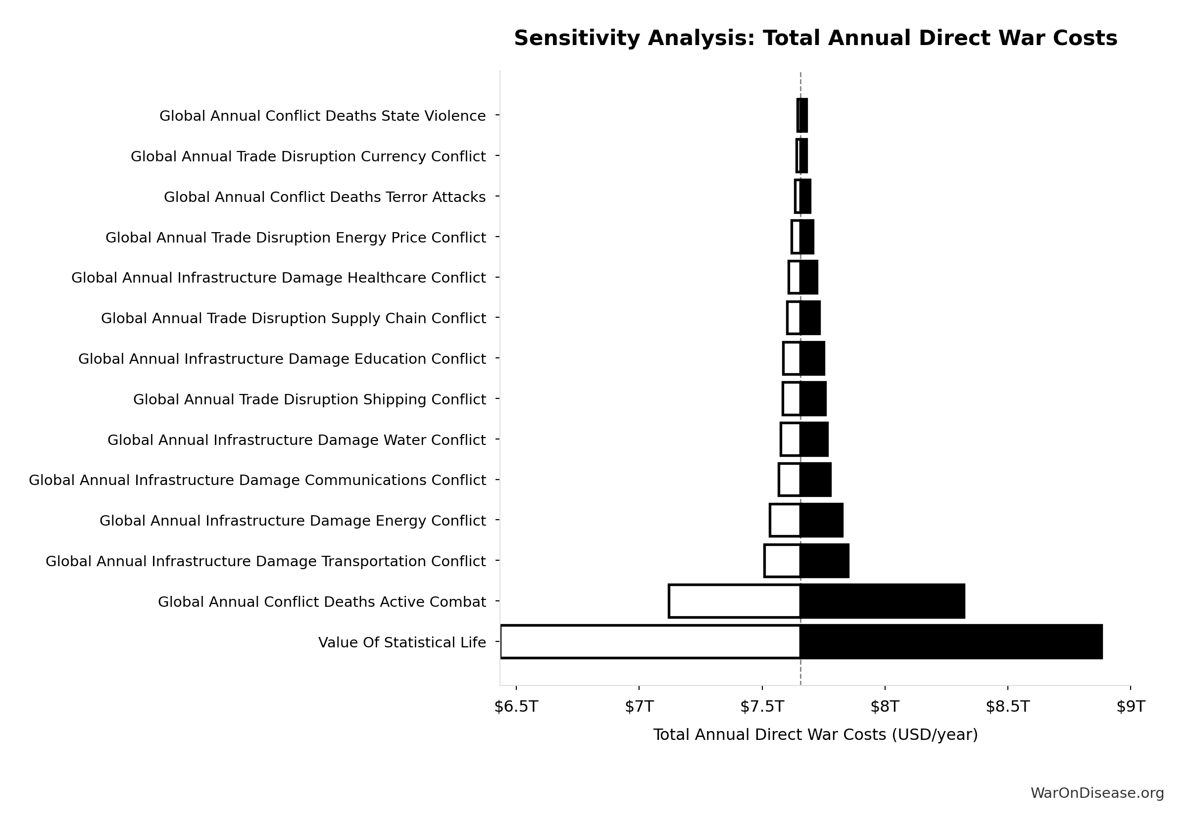
Sensitivity Analysis
Sensitivity Indices for Total Annual Direct War Costs
Regression-based sensitivity showing which inputs explain the most variance in the output.
| Input Parameter | Sensitivity Coefficient | Interpretation |
|---|---|---|
| Global Annual Human Life Losses Conflict | 0.7463 | Strong driver |
| Global Annual Infrastructure Destruction Conflict | 0.3211 | Moderate driver |
| Global Annual Trade Disruption Conflict | 0.1057 | Weak driver |
Interpretation: Standardized coefficients show the change in output (in SD units) per 1 SD change in input. Values near ±1 indicate strong influence; values exceeding ±1 may occur with correlated inputs.
Monte Carlo Distribution
Simulation Results Summary: Total Annual Direct War Costs
| Statistic | Value |
|---|---|
| Baseline (deterministic) | $7.66T |
| Mean (expected value) | $7.62T |
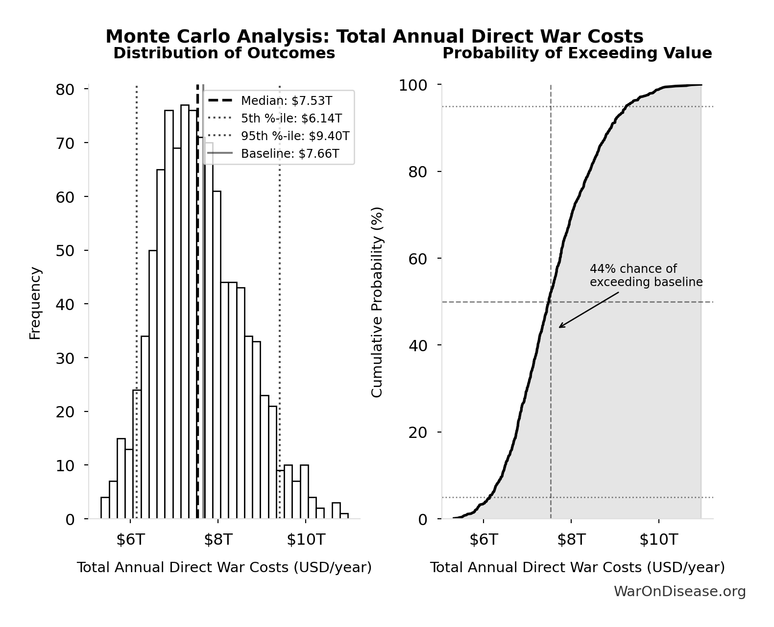
| Median (50th percentile) | $7.53T |
| Standard Deviation | $992B |
| 90% Confidence Interval | [$6.14T, $9.40T] |
The histogram shows the distribution of Total Annual Direct War Costs across 10,000 Monte Carlo simulations. The CDF (right) shows the probability of the outcome exceeding any given value, which is useful for risk assessment.
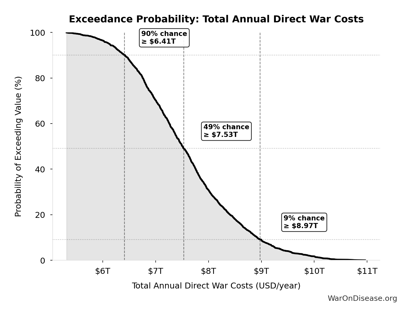
Exceedance Probability
This exceedance probability chart shows the likelihood that Total Annual Direct War Costs will exceed any given threshold. Higher curves indicate more favorable outcomes with greater certainty.
Total Annual Indirect War Costs: $3.70T
Total annual indirect war costs (opportunity cost + veterans + refugees + environment + mental health + lost productivity)
Inputs:
- Annual Environmental Damage and Restoration Costs from Conflict 📊: $100B (95% CI: $70B - $140B)
- Annual Lost Economic Growth from Military Spending Opportunity Cost 📊: $2.72T (95% CI: $1.90T - $3.80T)
- Annual Lost Productivity from Conflict Casualties 📊: $300B (95% CI: $210B - $420B)
- Annual PTSD and Mental Health Costs from Conflict 📊: $232B (95% CI: $162B - $325B)
- Annual Refugee Support Costs 📊: $150B (95% CI: $105B - $210B)
- Annual Veteran Healthcare Costs 📊: $200B (95% CI: $140B - $280B)
\[ \begin{gathered} Cost_{war,indirect} \\ = Damage_{env} + Loss_{growth,mil} + Loss_{capital,conflict} \\ + Cost_{psych} + Cost_{refugee} + Cost_{vet} \\ = \$100B + \$2.72T + \$300B + \$232B + \$150B + \$200B \\ = \$3.7T \end{gathered} \]
✓ High confidence
Sensitivity Analysis
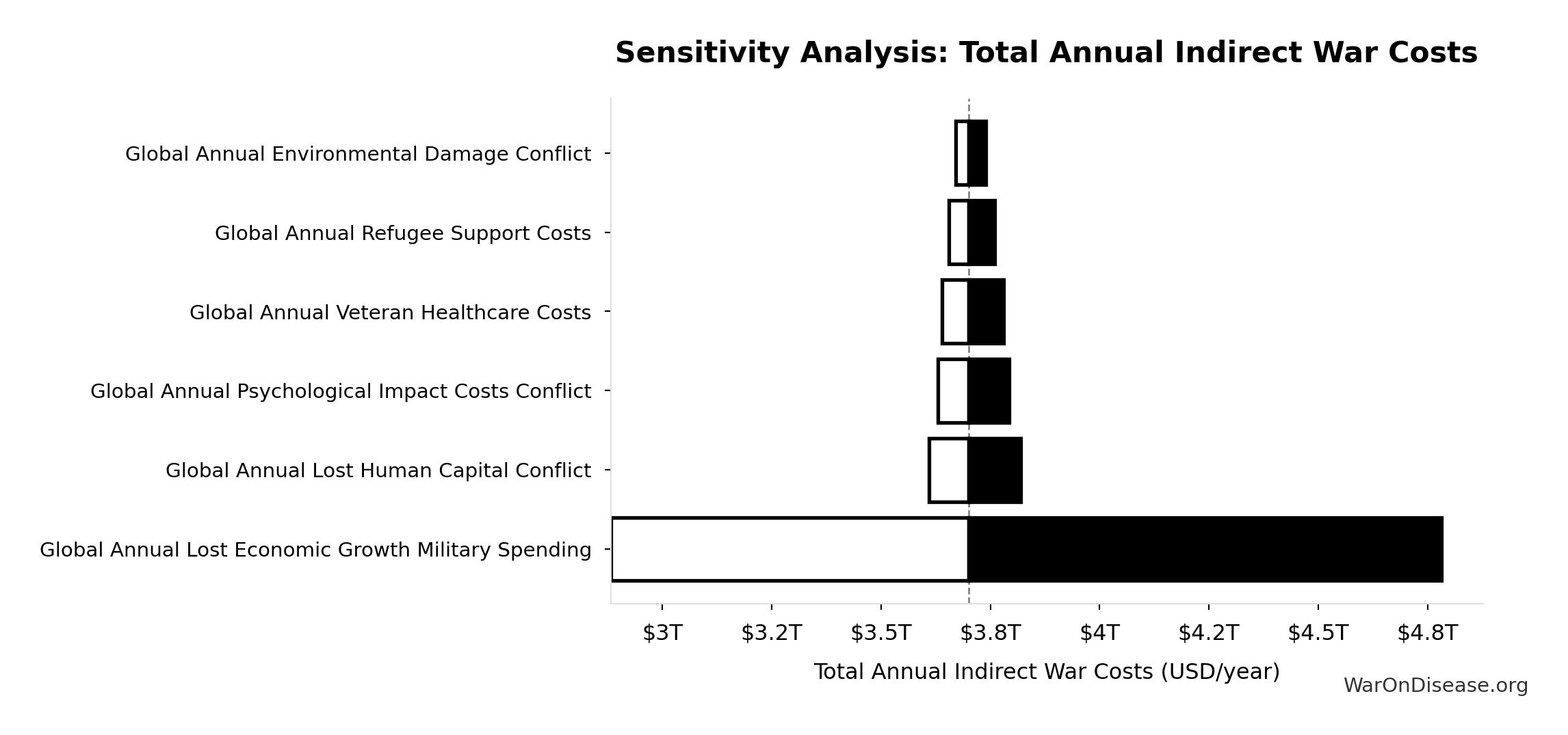
Sensitivity Indices for Total Annual Indirect War Costs
Regression-based sensitivity showing which inputs explain the most variance in the output.
| Input Parameter | Sensitivity Coefficient | Interpretation |
|---|---|---|
| Global Annual Refugee Support Costs | 3.5996 | Strong driver |
| Global Annual Lost Human Capital Conflict | -1.9754 | Strong driver |
| Global Annual Environmental Damage Conflict | -1.4754 | Strong driver |
| Global Annual Lost Economic Growth Military Spending | 0.7342 | Strong driver |
| Global Annual Psychological Impact Costs Conflict | 0.0630 | Minimal effect |
| Global Annual Veteran Healthcare Costs | 0.0541 | Minimal effect |
Interpretation: Standardized coefficients show the change in output (in SD units) per 1 SD change in input. Values near ±1 indicate strong influence; values exceeding ±1 may occur with correlated inputs.
Monte Carlo Distribution
Simulation Results Summary: Total Annual Indirect War Costs
| Statistic | Value |
|---|---|
| Baseline (deterministic) | $3.70T |
| Mean (expected value) | $3.69T |
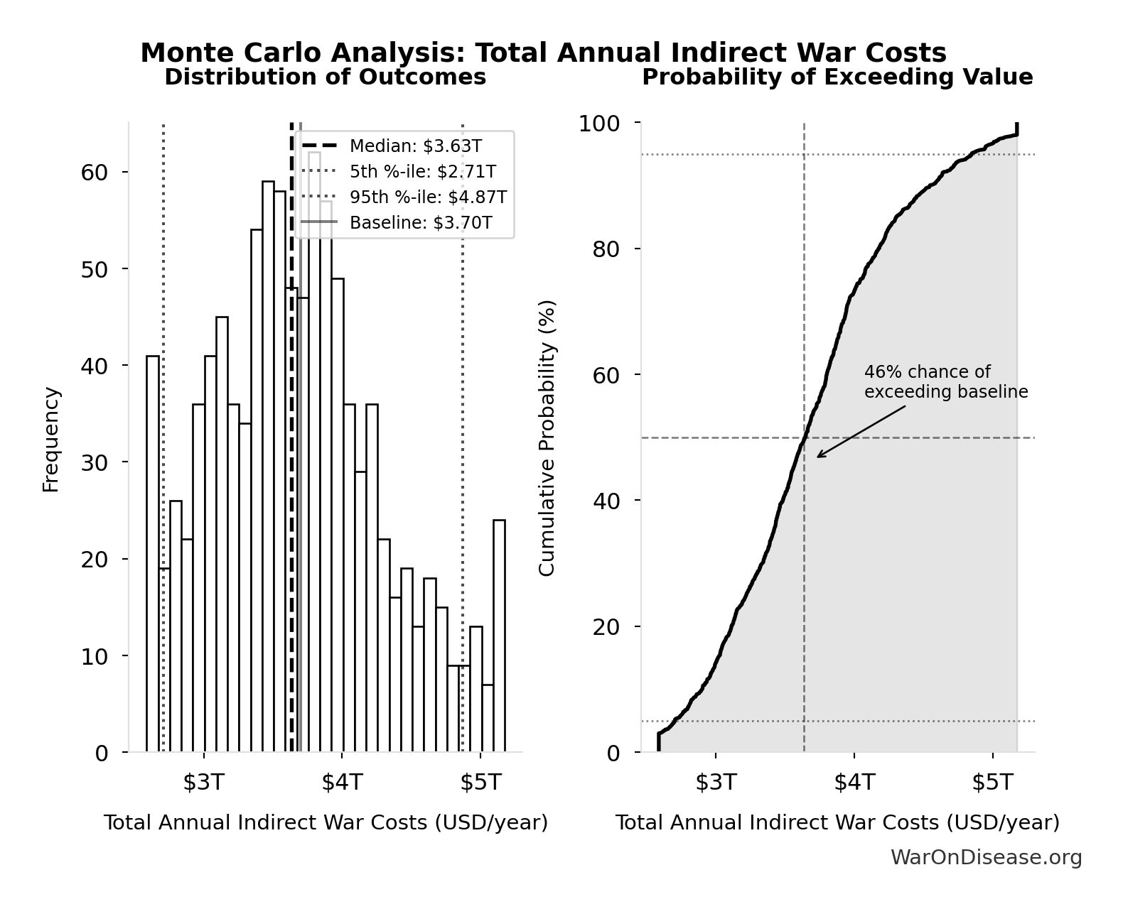
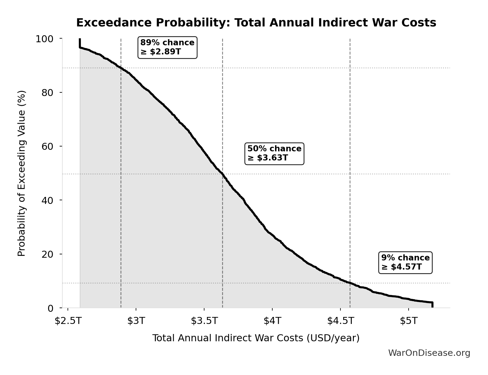
| Median (50th percentile) | $3.63T |
| Standard Deviation | $628B |
| 90% Confidence Interval | [$2.71T, $4.87T] |
The histogram shows the distribution of Total Annual Indirect War Costs across 10,000 Monte Carlo simulations. The CDF (right) shows the probability of the outcome exceeding any given value, which is useful for risk assessment.
Exceedance Probability
This exceedance probability chart shows the likelihood that Total Annual Indirect War Costs will exceed any given threshold. Higher curves indicate more favorable outcomes with greater certainty.
IAB Mechanism Benefit-Cost Ratio: 230:1
Benefit-Cost Ratio of the IAB mechanism itself
Inputs:
- 1% treaty Basic Annual Benefits (Peace + R&D Savings) 🔢: $172B
- IAB Mechanism Annual Cost (High Estimate): $750M (95% CI: $160M - $750M)
\[ \begin{gathered} BCR_{IAB} = \frac{Benefit_{peace+RD}}{Cost_{IAB,ann}} = \frac{\$172B}{\$750M} = 230 \\[0.5em] \text{where } Benefit_{peace+RD} \\ = Benefit_{peace,soc} + Benefit_{RD,ann} \\ = \$114B + \$58.6B \\ = \$172B \\[0.5em] \text{where } Benefit_{peace,soc} \\ = Cost_{war,total} \times Reduce_{treaty} \\ = \$11.4T \times 1\% \\ = \$114B \\[0.5em] \text{where } Cost_{war,total} \\ = Cost_{war,direct} + Cost_{war,indirect} \\ = \$7.66T + \$3.7T \\ = \$11.4T \\[0.5em] \text{where } Cost_{war,direct} \\ = Loss_{life,conflict} + Damage_{infra,total} \\ + Disruption_{trade} + Spending_{mil} \\ = \$2.45T + \$1.88T + \$616B + \$2.72T \\ = \$7.66T \\[0.5em] \text{where } Loss_{life,conflict} \\ = Cost_{combat,human} + Cost_{state,human} \\ + Cost_{terror,human} \\ = \$2.34T + \$27B + \$83B \\ = \$2.45T \\[0.5em] \text{where } Cost_{combat,human} \\ = Deaths_{combat} \times VSL \\ = 234{,}000 \times \$10M \\ = \$2.34T \\[0.5em] \text{where } Cost_{state,human} \\ = Deaths_{state} \times VSL \\ = 2{,}700 \times \$10M \\ = \$27B \\[0.5em] \text{where } Cost_{terror,human} \\ = Deaths_{terror} \times VSL \\ = 8{,}300 \times \$10M \\ = \$83B \\[0.5em] \text{where } Damage_{infra,total} \\ = Damage_{comms} + Damage_{edu} + Damage_{energy} \\ + Damage_{health} + Damage_{transport} \\ + Damage_{water} \\ = \$298B + \$234B + \$422B + \$166B + \$487B + \$268B \\ = \$1.88T \\[0.5em] \text{where } Disruption_{trade} \\ = Disruption_{currency} + Disruption_{energy} \\ + Disruption_{shipping} + Disruption_{supply} \\ = \$57.4B + \$125B + \$247B + \$187B \\ = \$616B \\[0.5em] \text{where } Cost_{war,indirect} \\ = Damage_{env} + Loss_{growth,mil} \\ + Loss_{capital,conflict} + Cost_{psych} \\ + Cost_{refugee} + Cost_{vet} \\ = \$100B + \$2.72T + \$300B + \$232B + \$150B + \$200B \\ = \$3.7T \\[0.5em] \text{where } Benefit_{RD,ann} \\ = Spending_{trials} \times Reduce_{pct} \\ = \$60B \times 97.7\% \\ = \$58.6B \\[0.5em] \text{where } Reduce_{pct} \\ = 1 - \frac{Cost_{pragmatic,pt}}{Cost_{P3,pt}} \\ = 1 - \frac{\$929}{\$41K} \\ = 97.7\% \end{gathered} \]
Methodology: https://iab.warondisease.org##welfare-analysis
✓ High confidence
Sensitivity Analysis
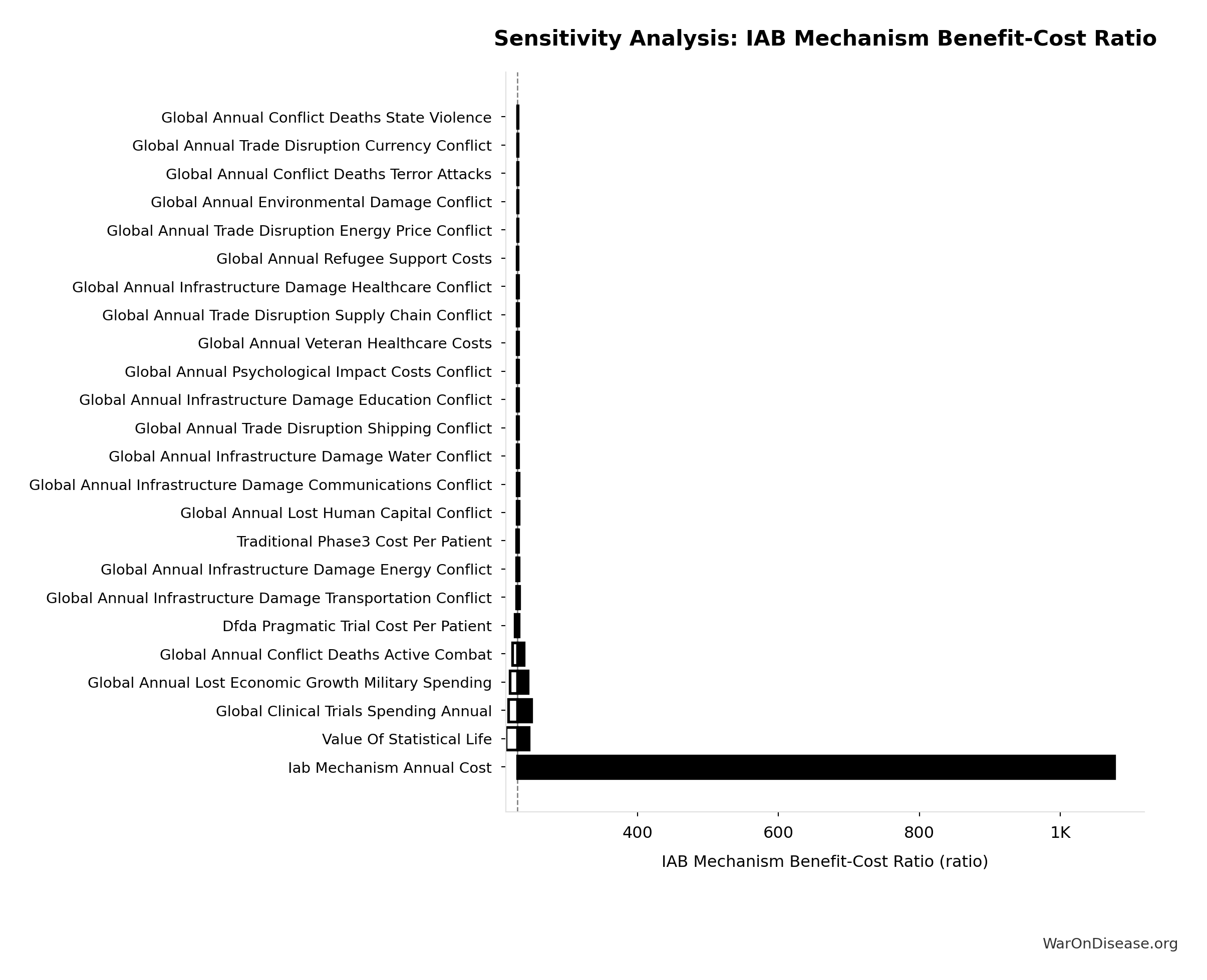
Sensitivity Indices for IAB Mechanism Benefit-Cost Ratio
Regression-based sensitivity showing which inputs explain the most variance in the output.
| Input Parameter | Sensitivity Coefficient | Interpretation |
|---|---|---|
| Treaty Peace Plus R&D Annual Benefits | 1.0000 | Strong driver |
Interpretation: Standardized coefficients show the change in output (in SD units) per 1 SD change in input. Values near ±1 indicate strong influence; values exceeding ±1 may occur with correlated inputs.
Monte Carlo Distribution
Simulation Results Summary: IAB Mechanism Benefit-Cost Ratio
| Statistic | Value |
|---|---|
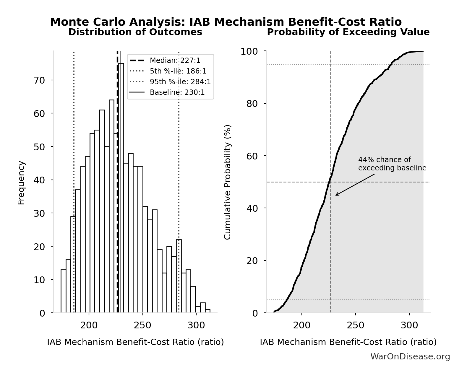
| Baseline (deterministic) | 230:1 |
| Mean (expected value) | 229:1 |
| Median (50th percentile) | 227:1 |
| Standard Deviation | 29.6:1 |
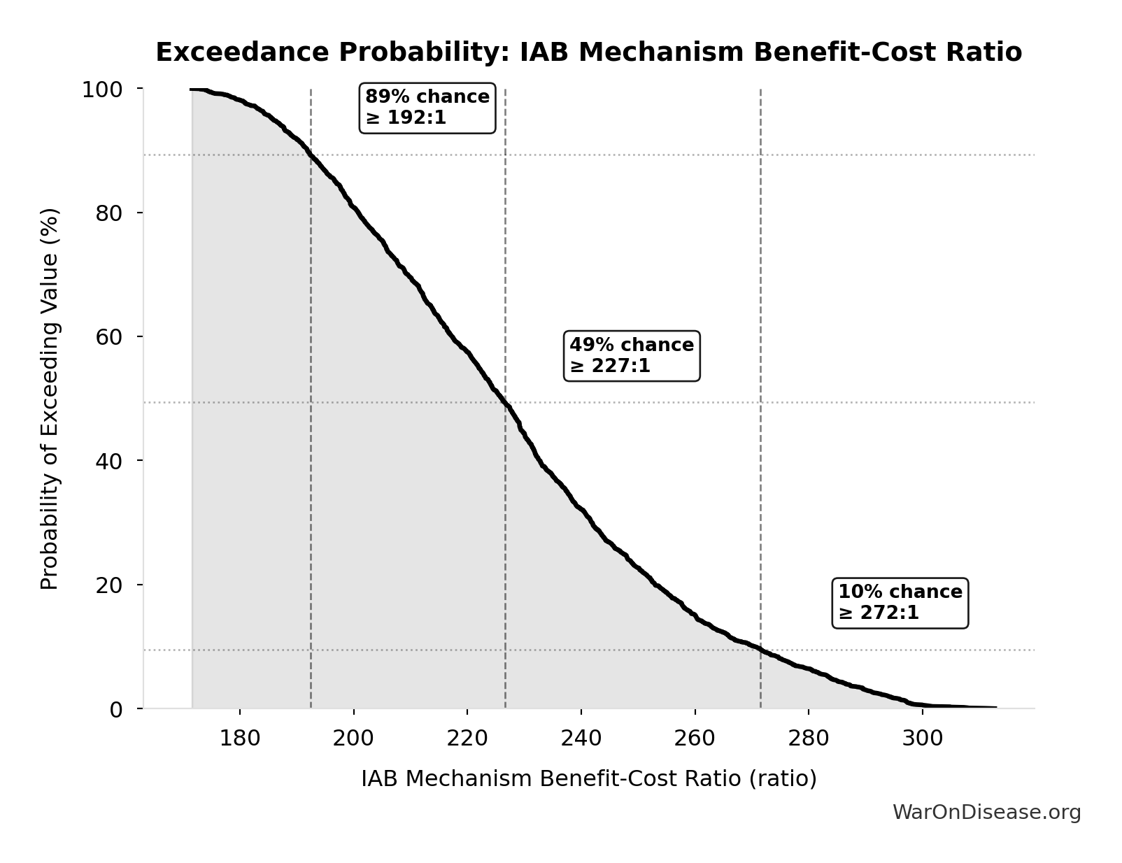
| 90% Confidence Interval | [186:1, 284:1] |
The histogram shows the distribution of IAB Mechanism Benefit-Cost Ratio across 10,000 Monte Carlo simulations. The CDF (right) shows the probability of the outcome exceeding any given value, which is useful for risk assessment.
Exceedance Probability
This exceedance probability chart shows the likelihood that IAB Mechanism Benefit-Cost Ratio will exceed any given threshold. Higher curves indicate more favorable outcomes with greater certainty.
Annual IAB Political Incentive Funding: $2.72B
Annual funding for IAB political incentive mechanism (independent expenditures supporting high-scoring politicians, post-office fellowship endowments, Public Good Score infrastructure)
Inputs:
- Annual Funding from 1% of Global Military Spending Redirected to DIH 🔢: $27.2B
- IAB Political Incentive Funding Percentage: 10%
\[ \begin{gathered} Funding_{political,ann} \\ = Funding_{treaty} \times Pct_{political} \\ = \$27.2B \times 10\% \\ = \$2.72B \\[0.5em] \text{where } Funding_{treaty} \\ = Spending_{mil} \times Reduce_{treaty} \\ = \$2.72T \times 1\% \\ = \$27.2B \end{gathered} \]
✓ High confidence
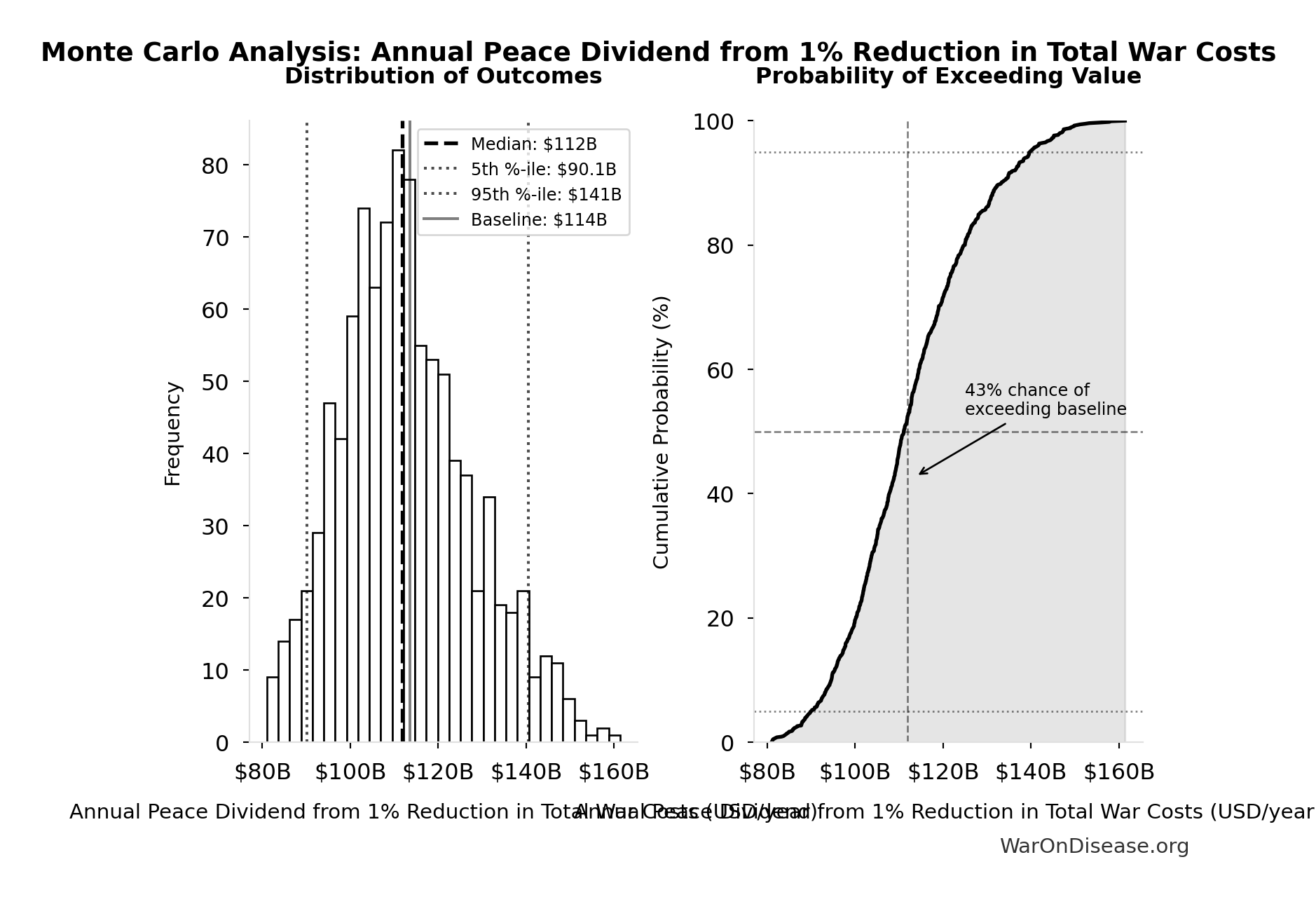
Annual Peace Dividend from 1% Reduction in Total War Costs: $114B
Annual peace dividend from 1% reduction in total war costs (theoretical maximum at ε=1.0)
Inputs:
- Total Annual Cost of War Worldwide 🔢: $11.4T
- 1% Reduction in Military Spending/War Costs from Treaty: 1%
\[ \begin{gathered} Benefit_{peace,soc} \\ = Cost_{war,total} \times Reduce_{treaty} \\ = \$11.4T \times 1\% \\ = \$114B \\[0.5em] \text{where } Cost_{war,total} \\ = Cost_{war,direct} + Cost_{war,indirect} \\ = \$7.66T + \$3.7T \\ = \$11.4T \\[0.5em] \text{where } Cost_{war,direct} \\ = Loss_{life,conflict} + Damage_{infra,total} \\ + Disruption_{trade} + Spending_{mil} \\ = \$2.45T + \$1.88T + \$616B + \$2.72T \\ = \$7.66T \\[0.5em] \text{where } Loss_{life,conflict} \\ = Cost_{combat,human} + Cost_{state,human} \\ + Cost_{terror,human} \\ = \$2.34T + \$27B + \$83B \\ = \$2.45T \\[0.5em] \text{where } Cost_{combat,human} \\ = Deaths_{combat} \times VSL \\ = 234{,}000 \times \$10M \\ = \$2.34T \\[0.5em] \text{where } Cost_{state,human} \\ = Deaths_{state} \times VSL \\ = 2{,}700 \times \$10M \\ = \$27B \\[0.5em] \text{where } Cost_{terror,human} \\ = Deaths_{terror} \times VSL \\ = 8{,}300 \times \$10M \\ = \$83B \\[0.5em] \text{where } Damage_{infra,total} \\ = Damage_{comms} + Damage_{edu} + Damage_{energy} \\ + Damage_{health} + Damage_{transport} \\ + Damage_{water} \\ = \$298B + \$234B + \$422B + \$166B + \$487B + \$268B \\ = \$1.88T \\[0.5em] \text{where } Disruption_{trade} \\ = Disruption_{currency} + Disruption_{energy} \\ + Disruption_{shipping} + Disruption_{supply} \\ = \$57.4B + \$125B + \$247B + \$187B \\ = \$616B \\[0.5em] \text{where } Cost_{war,indirect} \\ = Damage_{env} + Loss_{growth,mil} \\ + Loss_{capital,conflict} + Cost_{psych} \\ + Cost_{refugee} + Cost_{vet} \\ = \$100B + \$2.72T + \$300B + \$232B + \$150B + \$200B \\ = \$3.7T \end{gathered} \]
✓ High confidence
Sensitivity Analysis
Sensitivity Indices for Annual Peace Dividend from 1% Reduction in Total War Costs
Regression-based sensitivity showing which inputs explain the most variance in the output.
| Input Parameter | Sensitivity Coefficient | Interpretation |
|---|---|---|
| Global Annual Direct Indirect War Cost | 1.0000 | Strong driver |
Interpretation: Standardized coefficients show the change in output (in SD units) per 1 SD change in input. Values near ±1 indicate strong influence; values exceeding ±1 may occur with correlated inputs.
Monte Carlo Distribution
Simulation Results Summary: Annual Peace Dividend from 1% Reduction in Total War Costs
| Statistic | Value |
|---|---|
| Baseline (deterministic) | $114B |
| Mean (expected value) | $113B |
| Median (50th percentile) | $112B |
| Standard Deviation | $15.1B |
| 90% Confidence Interval | [$90.1B, $141B] |
The histogram shows the distribution of Annual Peace Dividend from 1% Reduction in Total War Costs across 10,000 Monte Carlo simulations. The CDF (right) shows the probability of the outcome exceeding any given value, which is useful for risk assessment.
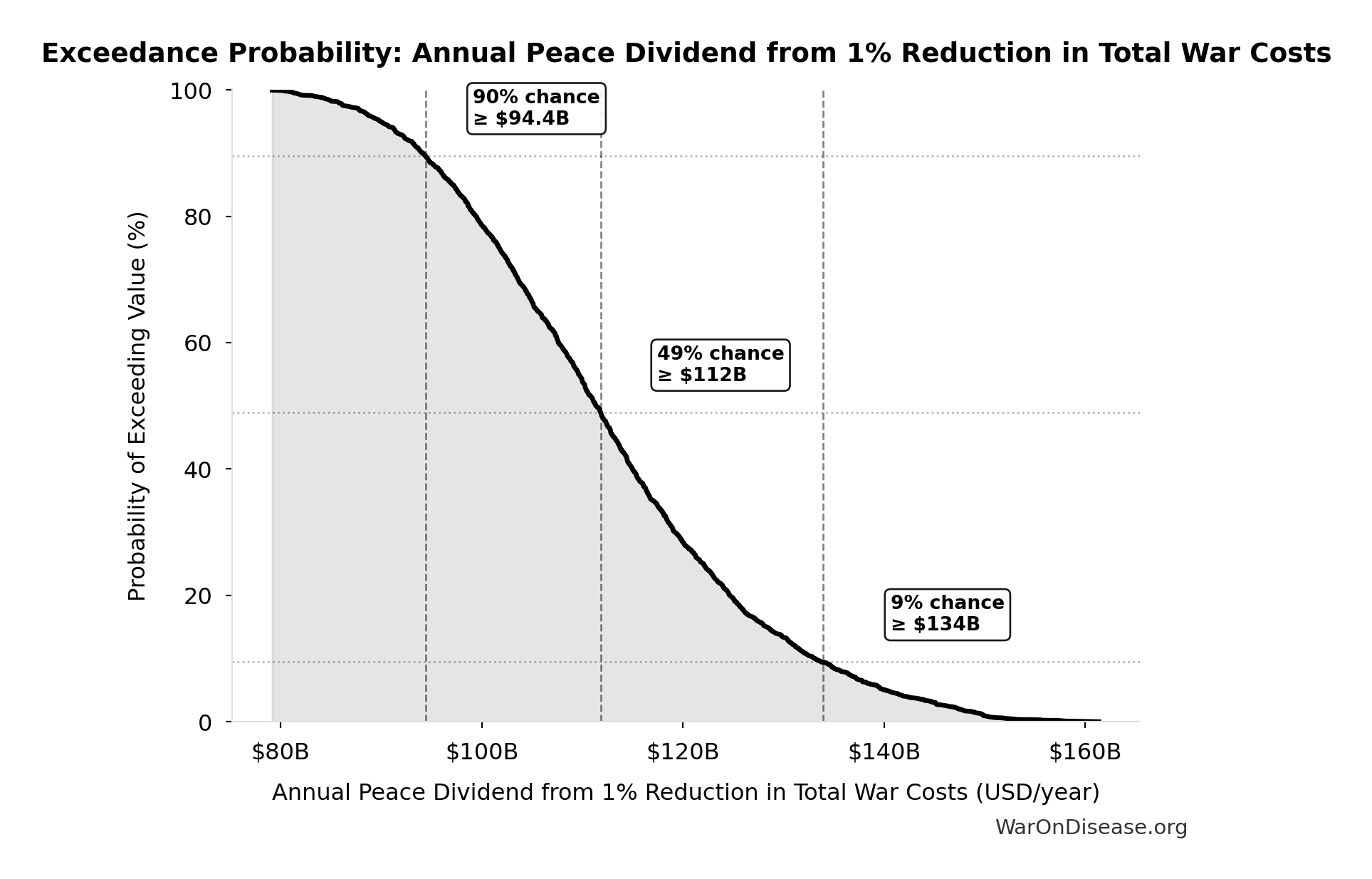
Exceedance Probability
This exceedance probability chart shows the likelihood that Annual Peace Dividend from 1% Reduction in Total War Costs will exceed any given threshold. Higher curves indicate more favorable outcomes with greater certainty.
Annual Funding from 1% of Global Military Spending Redirected to DIH: $27.2B
Annual funding from 1% of global military spending redirected to DIH
Inputs:
- Global Military Spending in 2024 📊: $2.72T
- 1% Reduction in Military Spending/War Costs from Treaty: 1%
\[ \begin{gathered} Funding_{treaty} \\ = Spending_{mil} \times Reduce_{treaty} \\ = \$2.72T \times 1\% \\ = \$27.2B \end{gathered} \]
✓ High confidence
Total 1% Treaty Campaign Cost: $1B
Total treaty campaign cost (100% VICTORY Incentive Alignment Bonds)
Inputs:
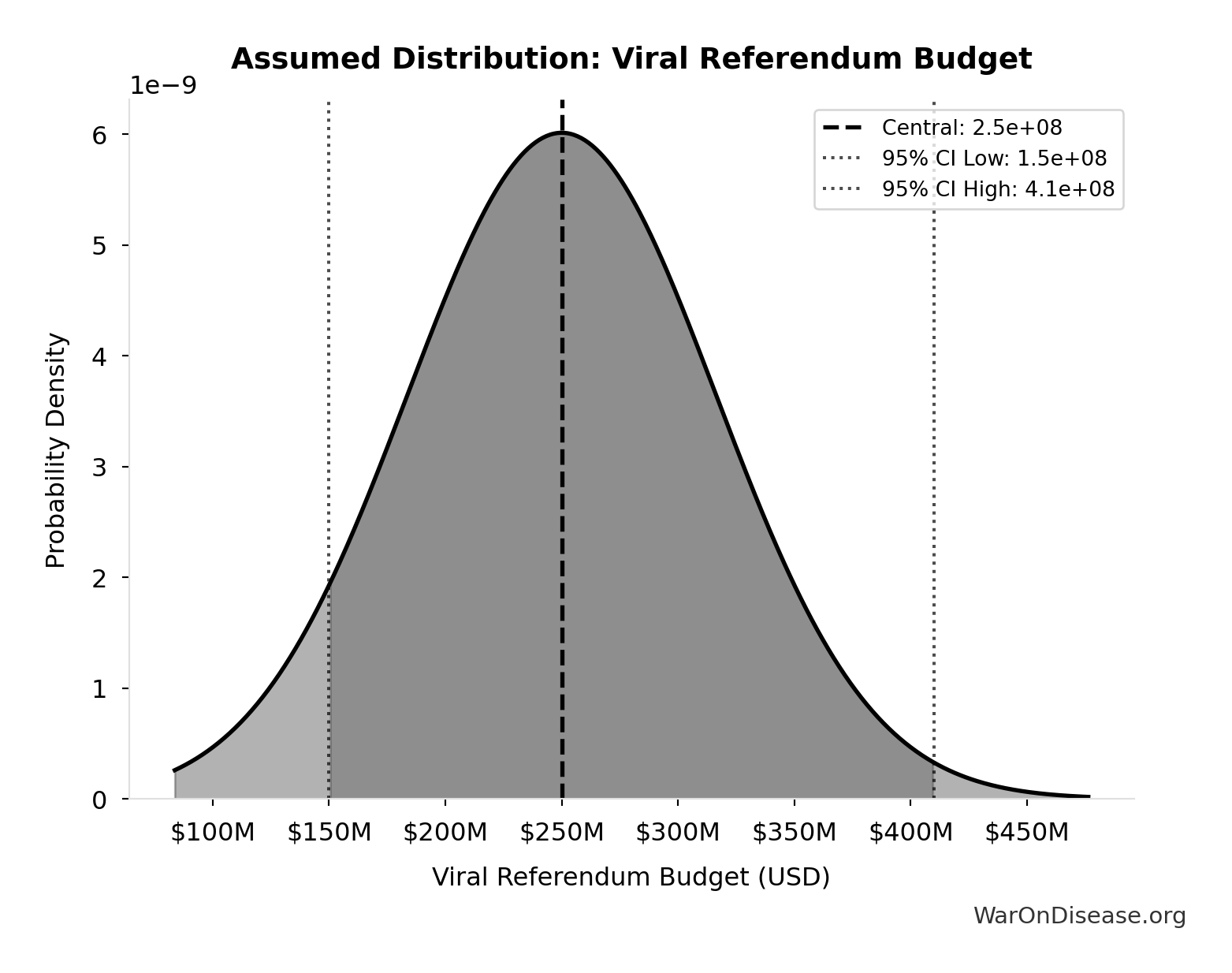
- Viral Referendum Budget: $250M (95% CI: $150M - $410M)
- Political Lobbying Campaign: Direct Lobbying, Super Pacs, Opposition Research, Staff, Legal/Compliance: $650M (95% CI: $325M - $1.30B)
- Reserve Fund / Contingency Buffer: $100M (95% CI: $20M - $150M)
\[ \begin{gathered} Cost_{campaign} \\ = Budget_{viral,base} + Budget_{lobby,treaty} \\ + Budget_{reserve} \\ = \$250M + \$650M + \$100M \\ = \$1B \end{gathered} \]
✓ High confidence
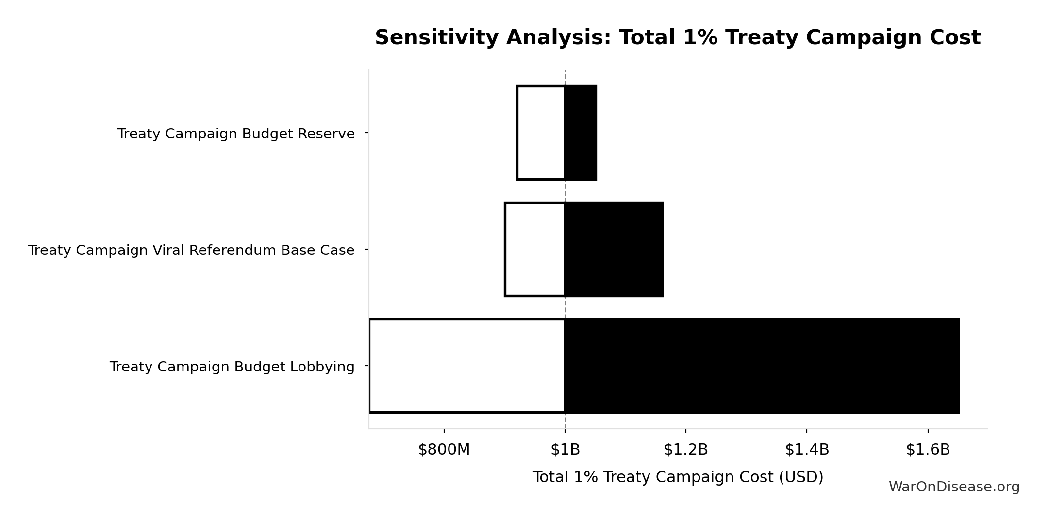
Sensitivity Analysis
Sensitivity Indices for Total 1% Treaty Campaign Cost
Regression-based sensitivity showing which inputs explain the most variance in the output.
| Input Parameter | Sensitivity Coefficient | Interpretation |
|---|---|---|
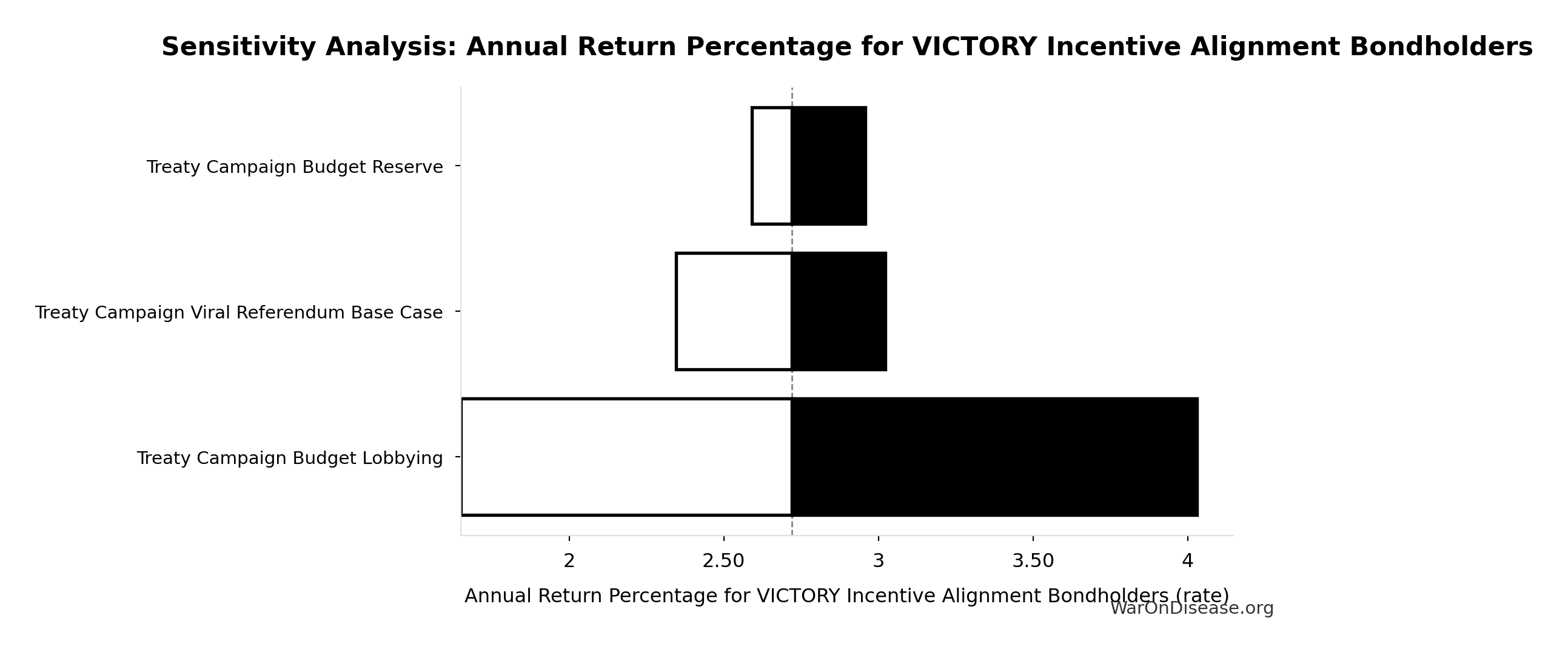
| Treaty Campaign Budget Lobbying | 0.9016 | Strong driver |
| Treaty Campaign Budget Reserve | 0.1026 | Weak driver |
Interpretation: Standardized coefficients show the change in output (in SD units) per 1 SD change in input. Values near ±1 indicate strong influence; values exceeding ±1 may occur with correlated inputs.
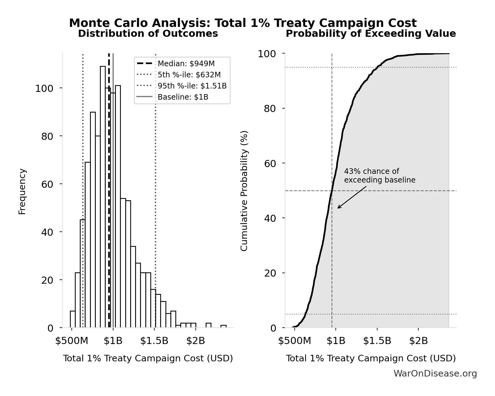
Monte Carlo Distribution
Simulation Results Summary: Total 1% Treaty Campaign Cost
| Statistic | Value |
|---|---|
| Baseline (deterministic) | $1B |
| Mean (expected value) | $996M |
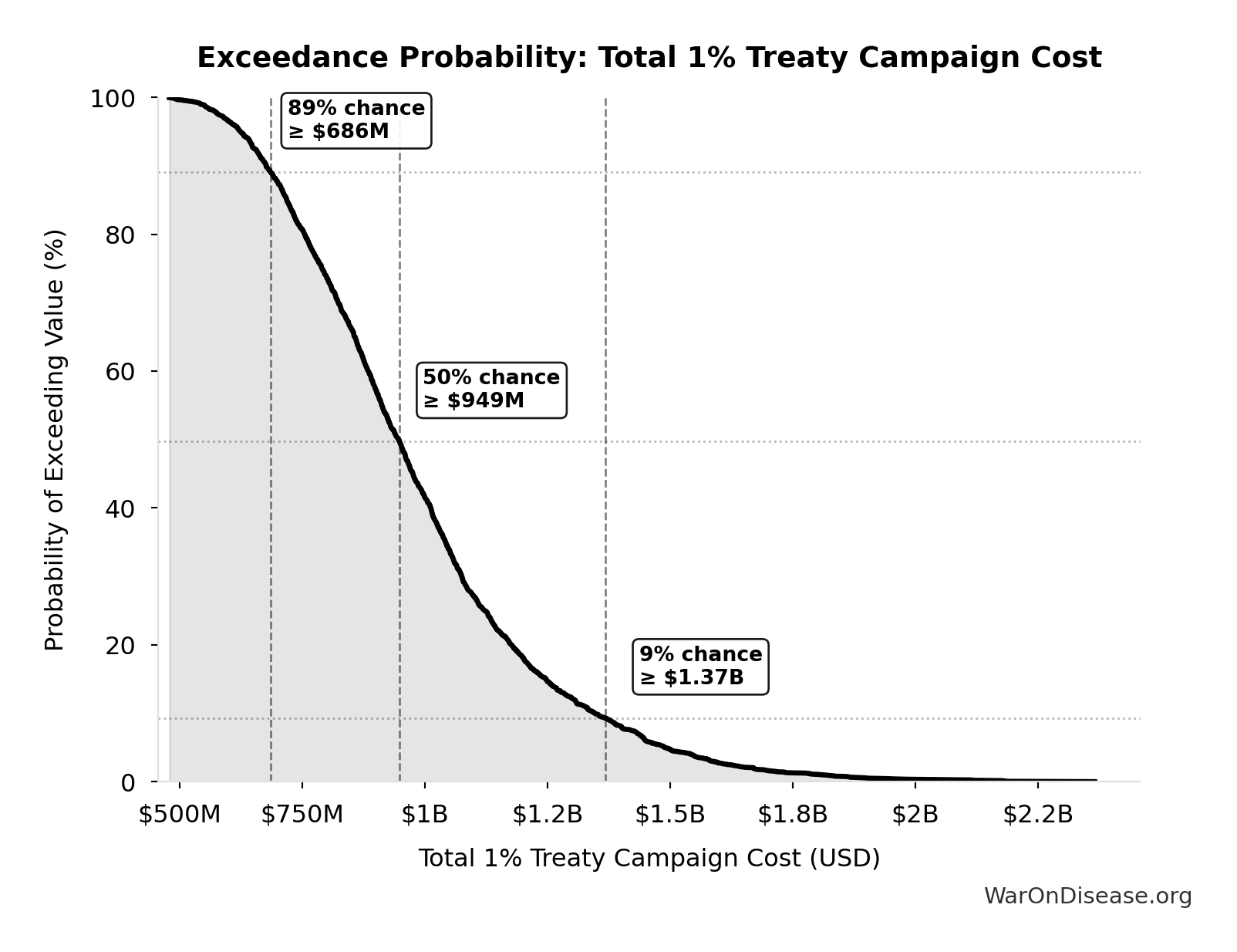
| Median (50th percentile) | $949M |
| Standard Deviation | $276M |
| 90% Confidence Interval | [$632M, $1.51B] |
The histogram shows the distribution of Total 1% Treaty Campaign Cost across 10,000 Monte Carlo simulations. The CDF (right) shows the probability of the outcome exceeding any given value, which is useful for risk assessment.
Exceedance Probability
This exceedance probability chart shows the likelihood that Total 1% Treaty Campaign Cost will exceed any given threshold. Higher curves indicate more favorable outcomes with greater certainty.
1% treaty Basic Annual Benefits (Peace + R&D Savings): $172B
Basic annual benefits: peace dividend + Decentralized Framework for Drug Assessment R&D savings only (2 of 8 benefit categories, excludes regulatory delay value)
Inputs:
- Annual Peace Dividend from 1% Reduction in Total War Costs 🔢: $114B
- Decentralized Framework for Drug Assessment Annual Benefit: R&D Savings 🔢: $58.6B
\[ \begin{gathered} Benefit_{peace+RD} \\ = Benefit_{peace,soc} + Benefit_{RD,ann} \\ = \$114B + \$58.6B \\ = \$172B \\[0.5em] \text{where } Benefit_{peace,soc} \\ = Cost_{war,total} \times Reduce_{treaty} \\ = \$11.4T \times 1\% \\ = \$114B \\[0.5em] \text{where } Cost_{war,total} \\ = Cost_{war,direct} + Cost_{war,indirect} \\ = \$7.66T + \$3.7T \\ = \$11.4T \\[0.5em] \text{where } Cost_{war,direct} \\ = Loss_{life,conflict} + Damage_{infra,total} \\ + Disruption_{trade} + Spending_{mil} \\ = \$2.45T + \$1.88T + \$616B + \$2.72T \\ = \$7.66T \\[0.5em] \text{where } Loss_{life,conflict} \\ = Cost_{combat,human} + Cost_{state,human} \\ + Cost_{terror,human} \\ = \$2.34T + \$27B + \$83B \\ = \$2.45T \\[0.5em] \text{where } Cost_{combat,human} \\ = Deaths_{combat} \times VSL \\ = 234{,}000 \times \$10M \\ = \$2.34T \\[0.5em] \text{where } Cost_{state,human} \\ = Deaths_{state} \times VSL \\ = 2{,}700 \times \$10M \\ = \$27B \\[0.5em] \text{where } Cost_{terror,human} \\ = Deaths_{terror} \times VSL \\ = 8{,}300 \times \$10M \\ = \$83B \\[0.5em] \text{where } Damage_{infra,total} \\ = Damage_{comms} + Damage_{edu} + Damage_{energy} \\ + Damage_{health} + Damage_{transport} \\ + Damage_{water} \\ = \$298B + \$234B + \$422B + \$166B + \$487B + \$268B \\ = \$1.88T \\[0.5em] \text{where } Disruption_{trade} \\ = Disruption_{currency} + Disruption_{energy} \\ + Disruption_{shipping} + Disruption_{supply} \\ = \$57.4B + \$125B + \$247B + \$187B \\ = \$616B \\[0.5em] \text{where } Cost_{war,indirect} \\ = Damage_{env} + Loss_{growth,mil} \\ + Loss_{capital,conflict} + Cost_{psych} \\ + Cost_{refugee} + Cost_{vet} \\ = \$100B + \$2.72T + \$300B + \$232B + \$150B + \$200B \\ = \$3.7T \\[0.5em] \text{where } Benefit_{RD,ann} \\ = Spending_{trials} \times Reduce_{pct} \\ = \$60B \times 97.7\% \\ = \$58.6B \\[0.5em] \text{where } Reduce_{pct} \\ = 1 - \frac{Cost_{pragmatic,pt}}{Cost_{P3,pt}} \\ = 1 - \frac{\$929}{\$41K} \\ = 97.7\% \end{gathered} \]
✓ High confidence
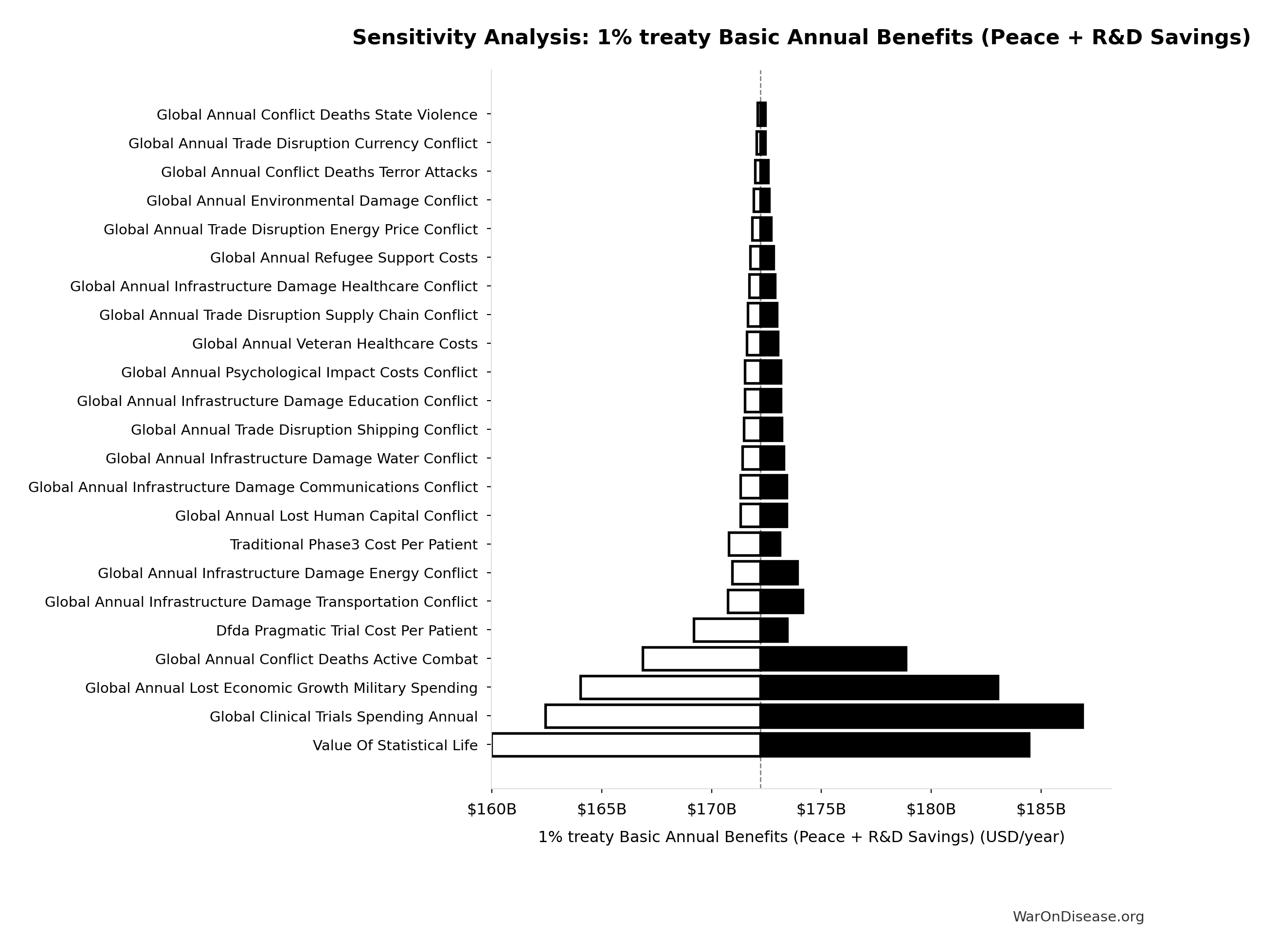
Sensitivity Analysis
Sensitivity Indices for 1% treaty Basic Annual Benefits (Peace + R&D Savings)
Regression-based sensitivity showing which inputs explain the most variance in the output.
| Input Parameter | Sensitivity Coefficient | Interpretation |
|---|---|---|
| Peace Dividend Annual Societal Benefit | 0.6828 | Strong driver |
| dFDA Benefit R&D Only Annual | 0.3457 | Moderate driver |
Interpretation: Standardized coefficients show the change in output (in SD units) per 1 SD change in input. Values near ±1 indicate strong influence; values exceeding ±1 may occur with correlated inputs.
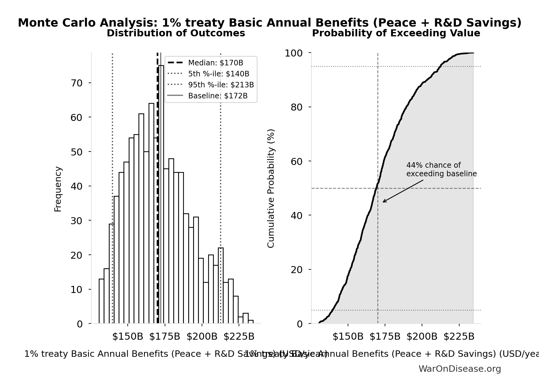
Monte Carlo Distribution
Simulation Results Summary: 1% treaty Basic Annual Benefits (Peace + R&D Savings)
| Statistic | Value |
|---|---|
| Baseline (deterministic) | $172B |
| Mean (expected value) | $172B |
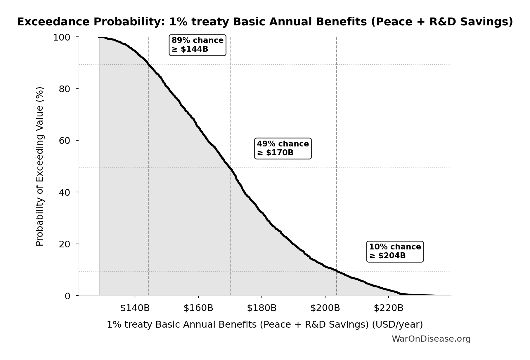
| Median (50th percentile) | $170B |
| Standard Deviation | $22.2B |
| 90% Confidence Interval | [$140B, $213B] |
The histogram shows the distribution of 1% treaty Basic Annual Benefits (Peace + R&D Savings) across 10,000 Monte Carlo simulations. The CDF (right) shows the probability of the outcome exceeding any given value, which is useful for risk assessment.
Exceedance Probability
This exceedance probability chart shows the likelihood that 1% treaty Basic Annual Benefits (Peace + R&D Savings) will exceed any given threshold. Higher curves indicate more favorable outcomes with greater certainty.
Annual VICTORY Incentive Alignment Bond Payout: $2.72B
Annual VICTORY Incentive Alignment Bond payout (treaty funding × bond percentage)
Inputs:
- Annual Funding from 1% of Global Military Spending Redirected to DIH 🔢: $27.2B
- Percentage of Captured Dividend Funding VICTORY Incentive Alignment Bonds: 10%
\[ \begin{gathered} Payout_{bond,ann} \\ = Funding_{treaty} \times Pct_{bond} \\ = \$27.2B \times 10\% \\ = \$2.72B \\[0.5em] \text{where } Funding_{treaty} \\ = Spending_{mil} \times Reduce_{treaty} \\ = \$2.72T \times 1\% \\ = \$27.2B \end{gathered} \]
✓ High confidence
Annual Return Percentage for VICTORY Incentive Alignment Bondholders: 272%
Annual return percentage for VICTORY Incentive Alignment Bondholders
Inputs:
\[ \begin{gathered} r_{bond} = \frac{Payout_{bond,ann}}{Cost_{campaign}} = \frac{\$2.72B}{\$1B} = 272\% \\[0.5em] \text{where } Payout_{bond,ann} \\ = Funding_{treaty} \times Pct_{bond} \\ = \$27.2B \times 10\% \\ = \$2.72B \\[0.5em] \text{where } Funding_{treaty} \\ = Spending_{mil} \times Reduce_{treaty} \\ = \$2.72T \times 1\% \\ = \$27.2B \\[0.5em] \text{where } Cost_{campaign} \\ = Budget_{viral,base} + Budget_{lobby,treaty} \\ + Budget_{reserve} \\ = \$250M + \$650M + \$100M \\ = \$1B \end{gathered} \]
✓ High confidence
Sensitivity Analysis
Sensitivity Indices for Annual Return Percentage for VICTORY Incentive Alignment Bondholders
Regression-based sensitivity showing which inputs explain the most variance in the output.
| Input Parameter | Sensitivity Coefficient | Interpretation |
|---|---|---|
| Treaty Campaign Total Cost | -0.9366 | Strong driver |
Interpretation: Standardized coefficients show the change in output (in SD units) per 1 SD change in input. Values near ±1 indicate strong influence; values exceeding ±1 may occur with correlated inputs.
Monte Carlo Distribution
Simulation Results Summary: Annual Return Percentage for VICTORY Incentive Alignment Bondholders
| Statistic | Value |
|---|---|
| Baseline (deterministic) | 272% |
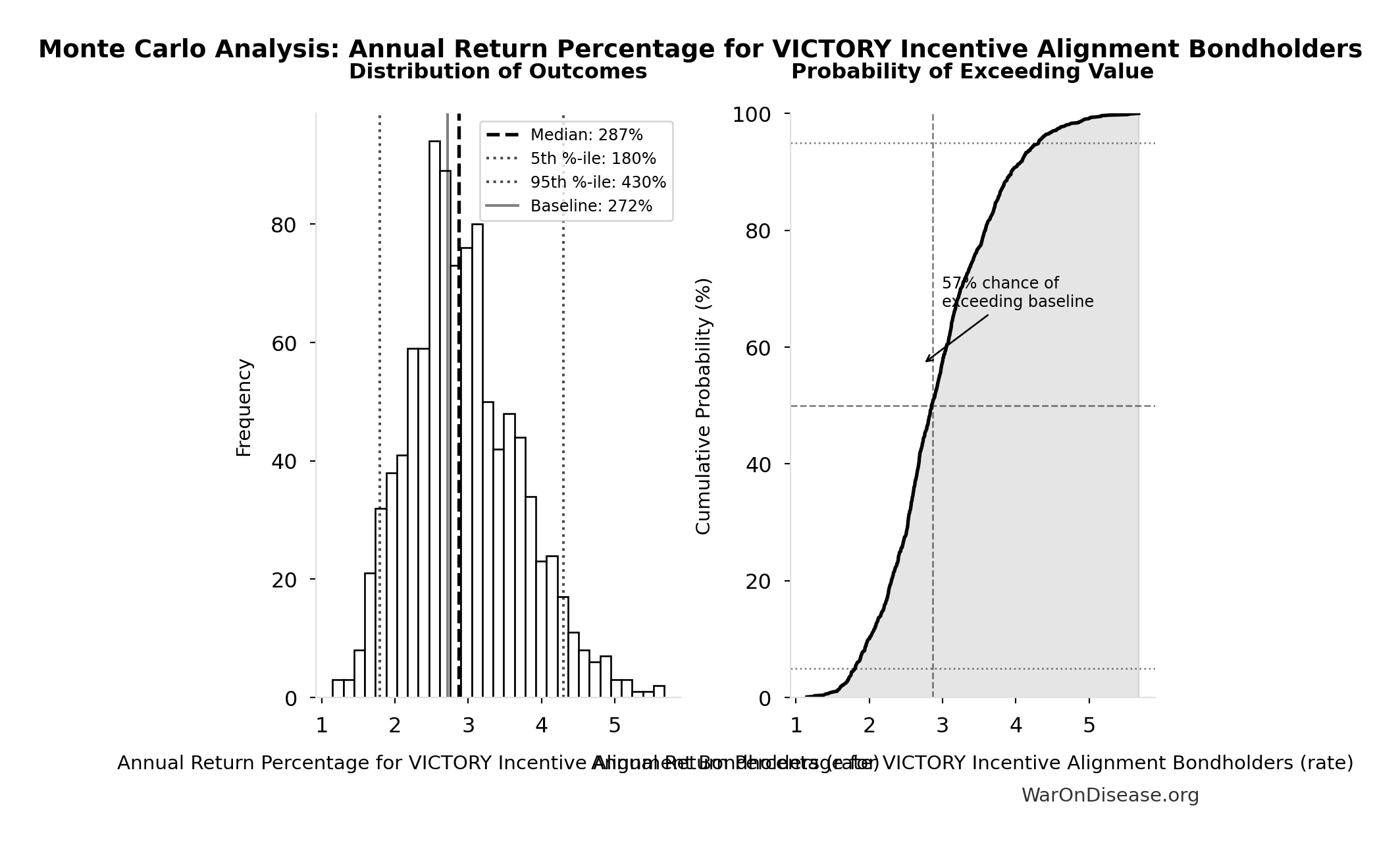
| Mean (expected value) | 293% |
| Median (50th percentile) | 287% |
| Standard Deviation | 76.3% |
| 90% Confidence Interval | [180%, 430%] |
The histogram shows the distribution of Annual Return Percentage for VICTORY Incentive Alignment Bondholders across 10,000 Monte Carlo simulations. The CDF (right) shows the probability of the outcome exceeding any given value, which is useful for risk assessment.
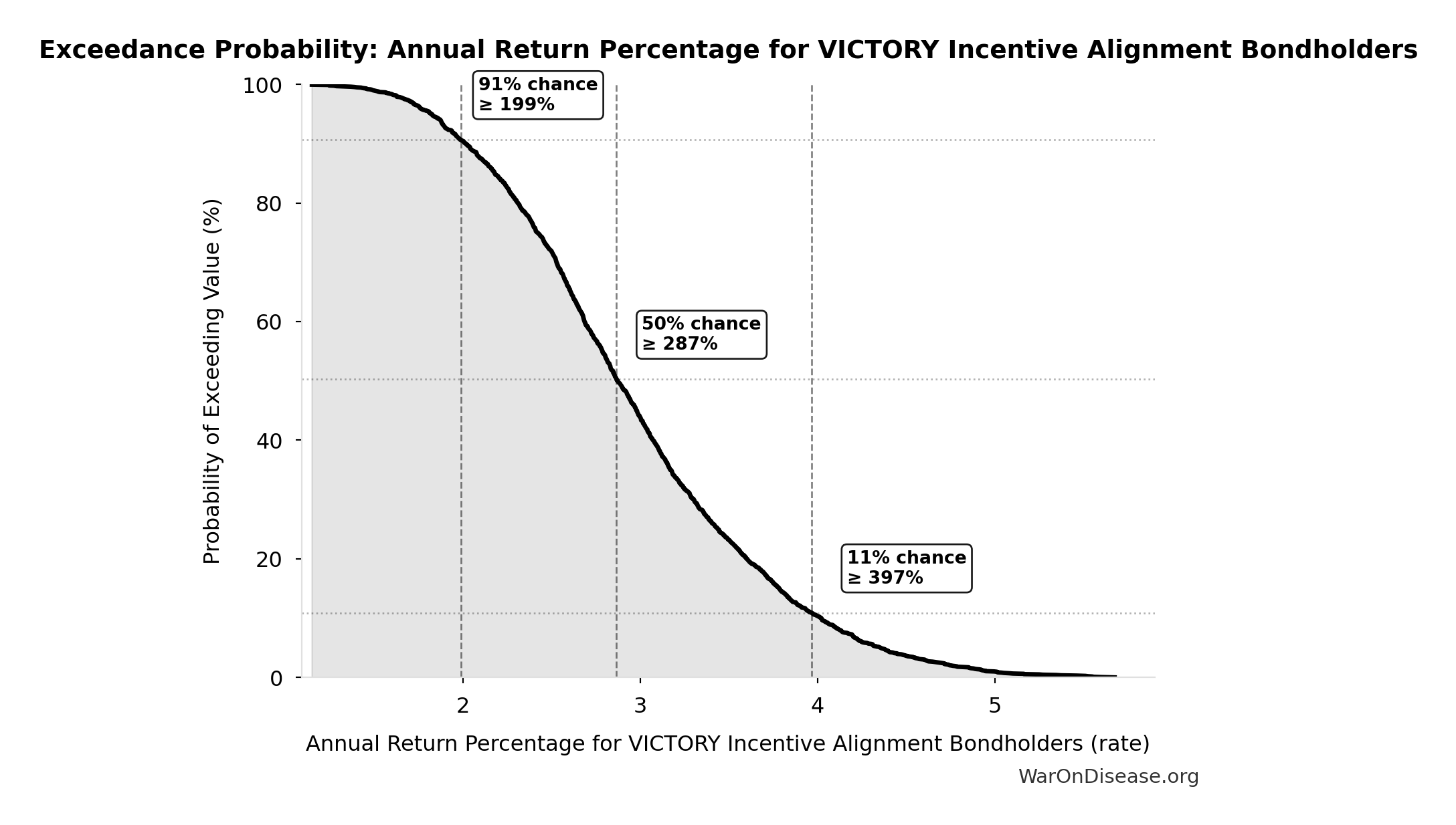
Exceedance Probability
This exceedance probability chart shows the likelihood that Annual Return Percentage for VICTORY Incentive Alignment Bondholders will exceed any given threshold. Higher curves indicate more favorable outcomes with greater certainty.
External Data Sources
Parameters sourced from peer-reviewed publications, institutional databases, and authoritative reports.
Average Annual Stock Market Return: 10%
dFDA Pragmatic Trial Cost per Patient: $929
dFDA pragmatic trial cost per patient. Uses ADAPTABLE trial ($929) as DELIBERATELY CONSERVATIVE central estimate. Harvard meta-analysis of 108 trials found median of only $97/patient - our estimate may overstate costs by 10x. Confidence interval spans meta-analysis median to complex chronic disease trials.
Source:1
Uncertainty Range
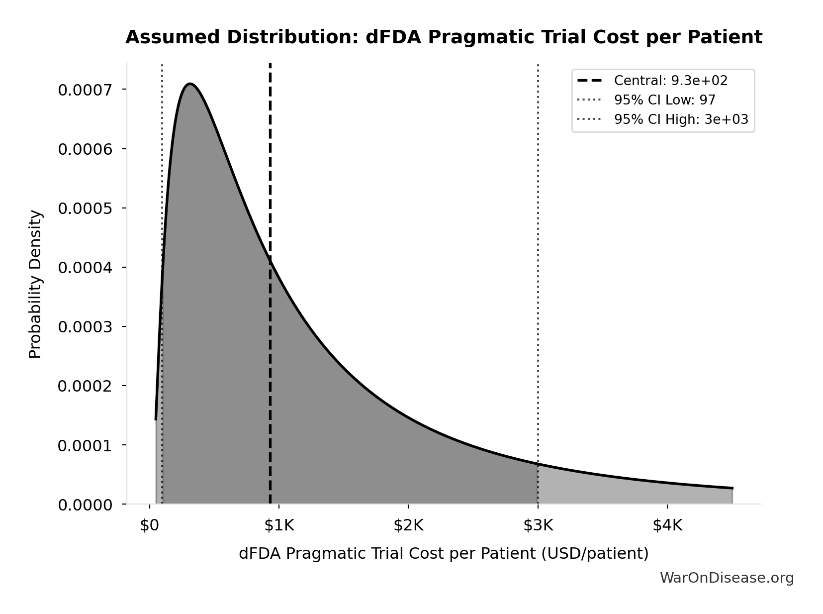
Technical: 95% CI: [$97, $3K] • Distribution: Lognormal
What this means: This estimate is highly uncertain. The true value likely falls between $97 and $3K (±156%). This represents a very wide range that our Monte Carlo simulations account for when calculating overall uncertainty in the results.
The lognormal distribution means values can’t go negative and have a longer tail toward higher values (common for costs and populations).
Input Distribution
This chart shows the assumed probability distribution for this parameter. The shaded region represents the 95% confidence interval where we expect the true value to fall.
~ Medium confidence
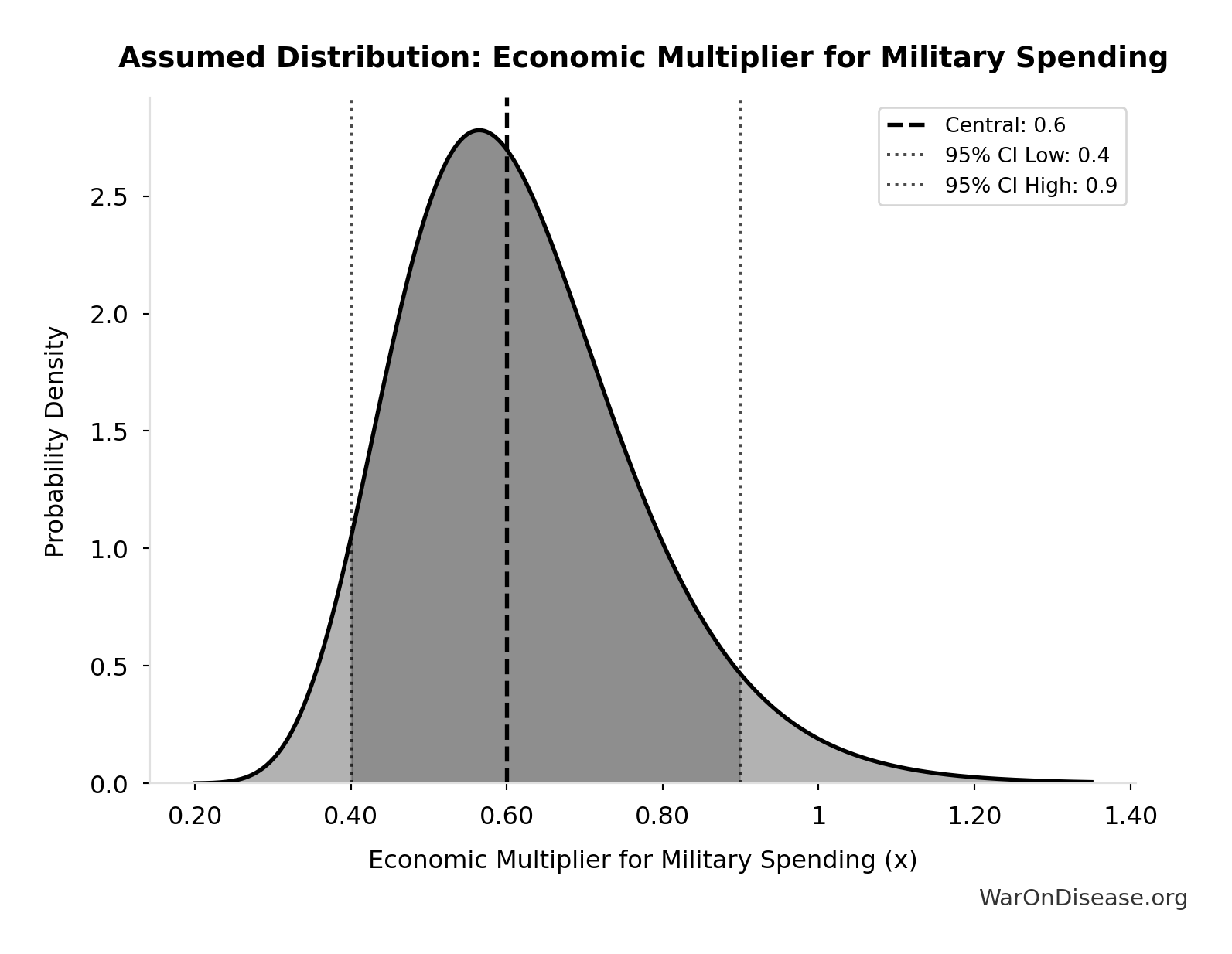
Economic Multiplier for Military Spending: 0.6x
Economic multiplier for military spending (0.6x ROI). Literature range 0.4-1.0×.
Source:26
Uncertainty Range
Technical: 95% CI: [0.4x, 0.9x] • Distribution: Lognormal
What this means: There’s significant uncertainty here. The true value likely falls between 0.4x and 0.9x (±42%). This represents a wide range that our Monte Carlo simulations account for when calculating overall uncertainty in the results.
The lognormal distribution means values can’t go negative and have a longer tail toward higher values (common for costs and populations).
Input Distribution
This chart shows the assumed probability distribution for this parameter. The shaded region represents the 95% confidence interval where we expect the true value to fall.
✓ High confidence
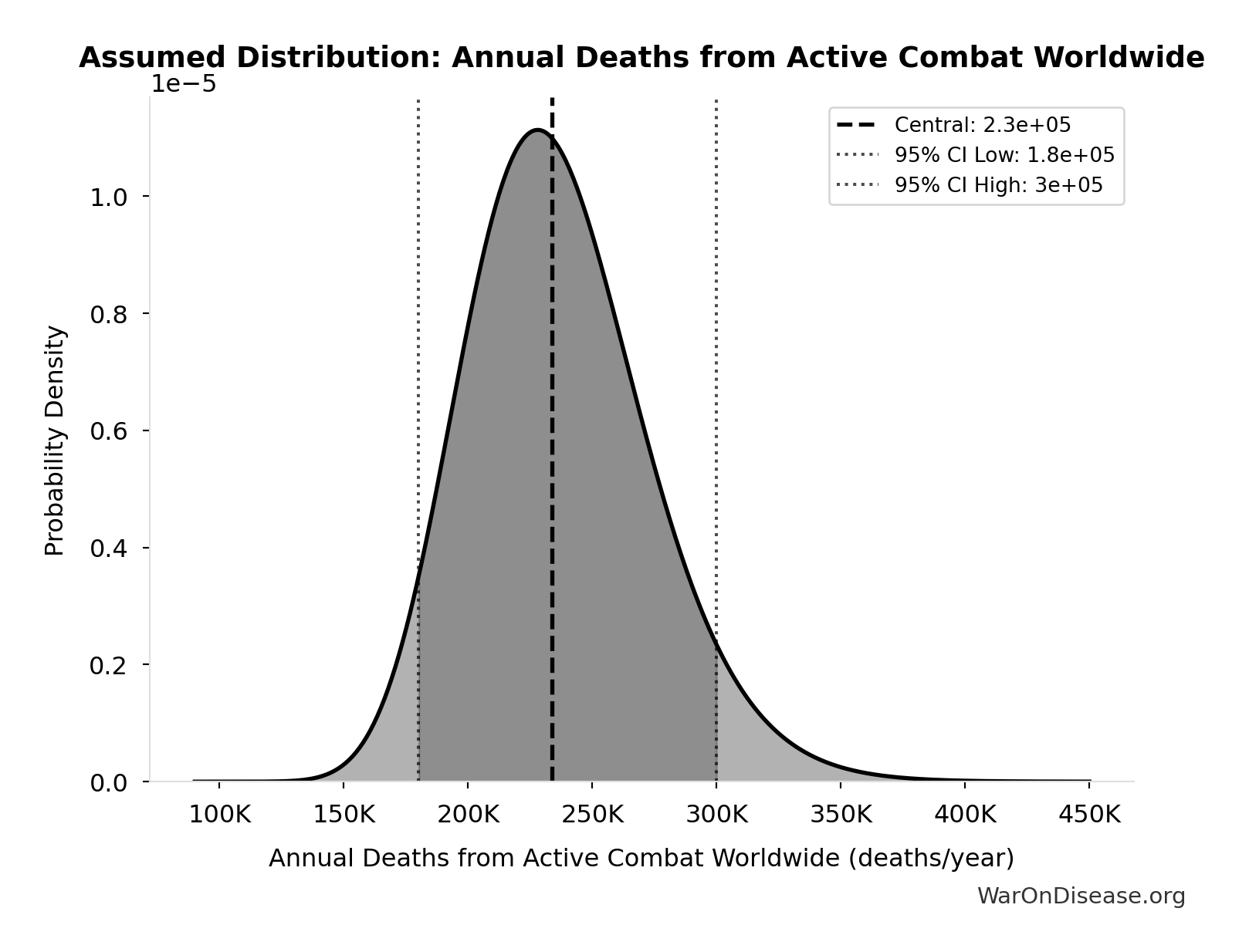
Annual Deaths from Active Combat Worldwide: 234k deaths/year
Annual deaths from active combat worldwide
Source:29
Uncertainty Range
Technical: 95% CI: [180k deaths/year, 300k deaths/year] • Distribution: Lognormal
What this means: There’s significant uncertainty here. The true value likely falls between 180k deaths/year and 300k deaths/year (±26%). This represents a wide range that our Monte Carlo simulations account for when calculating overall uncertainty in the results.
The lognormal distribution means values can’t go negative and have a longer tail toward higher values (common for costs and populations).
Input Distribution
This chart shows the assumed probability distribution for this parameter. The shaded region represents the 95% confidence interval where we expect the true value to fall.
✓ High confidence
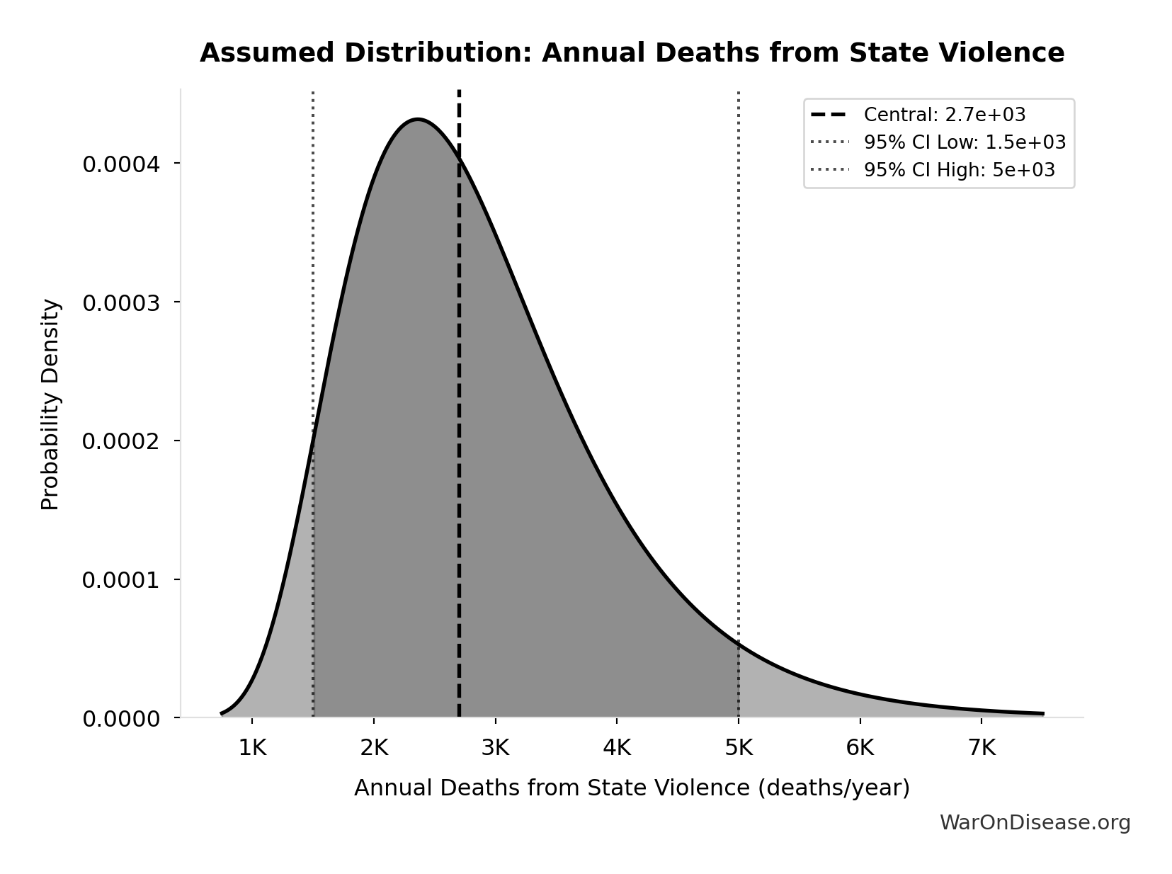
Annual Deaths from State Violence: 2.70k deaths/year
Annual deaths from state violence
Source:30
Uncertainty Range
Technical: 95% CI: [1.50k deaths/year, 5.00k deaths/year] • Distribution: Lognormal
What this means: This estimate is highly uncertain. The true value likely falls between 1.50k deaths/year and 5.00k deaths/year (±65%). This represents a very wide range that our Monte Carlo simulations account for when calculating overall uncertainty in the results.
The lognormal distribution means values can’t go negative and have a longer tail toward higher values (common for costs and populations).
Input Distribution
This chart shows the assumed probability distribution for this parameter. The shaded region represents the 95% confidence interval where we expect the true value to fall.
✓ High confidence
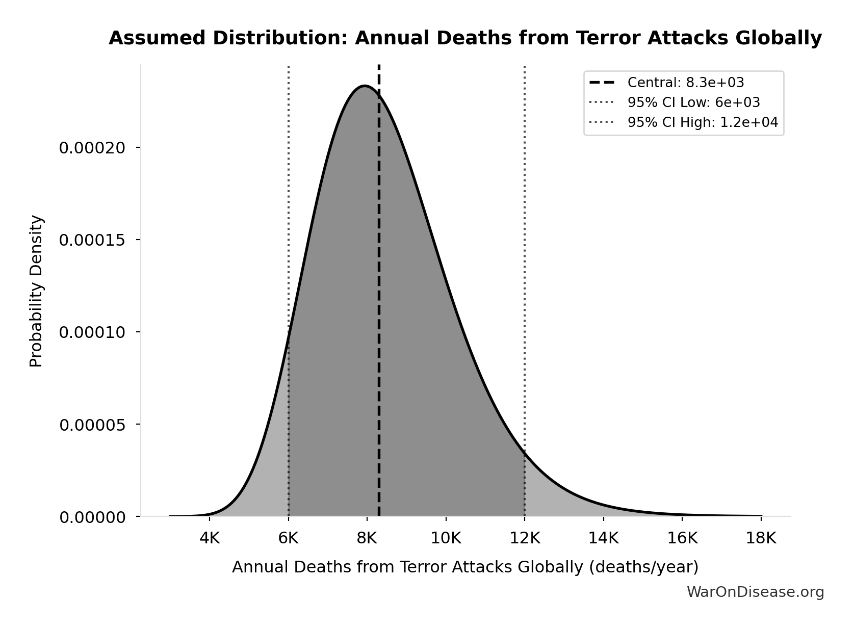
Annual Deaths from Terror Attacks Globally: 8.30k deaths/year
Annual deaths from terror attacks globally
Source:31
Uncertainty Range
Technical: 95% CI: [6.00k deaths/year, 12.0k deaths/year] • Distribution: Lognormal
What this means: There’s significant uncertainty here. The true value likely falls between 6.00k deaths/year and 12.0k deaths/year (±36%). This represents a wide range that our Monte Carlo simulations account for when calculating overall uncertainty in the results.
The lognormal distribution means values can’t go negative and have a longer tail toward higher values (common for costs and populations).
Input Distribution
This chart shows the assumed probability distribution for this parameter. The shaded region represents the 95% confidence interval where we expect the true value to fall.
✓ High confidence
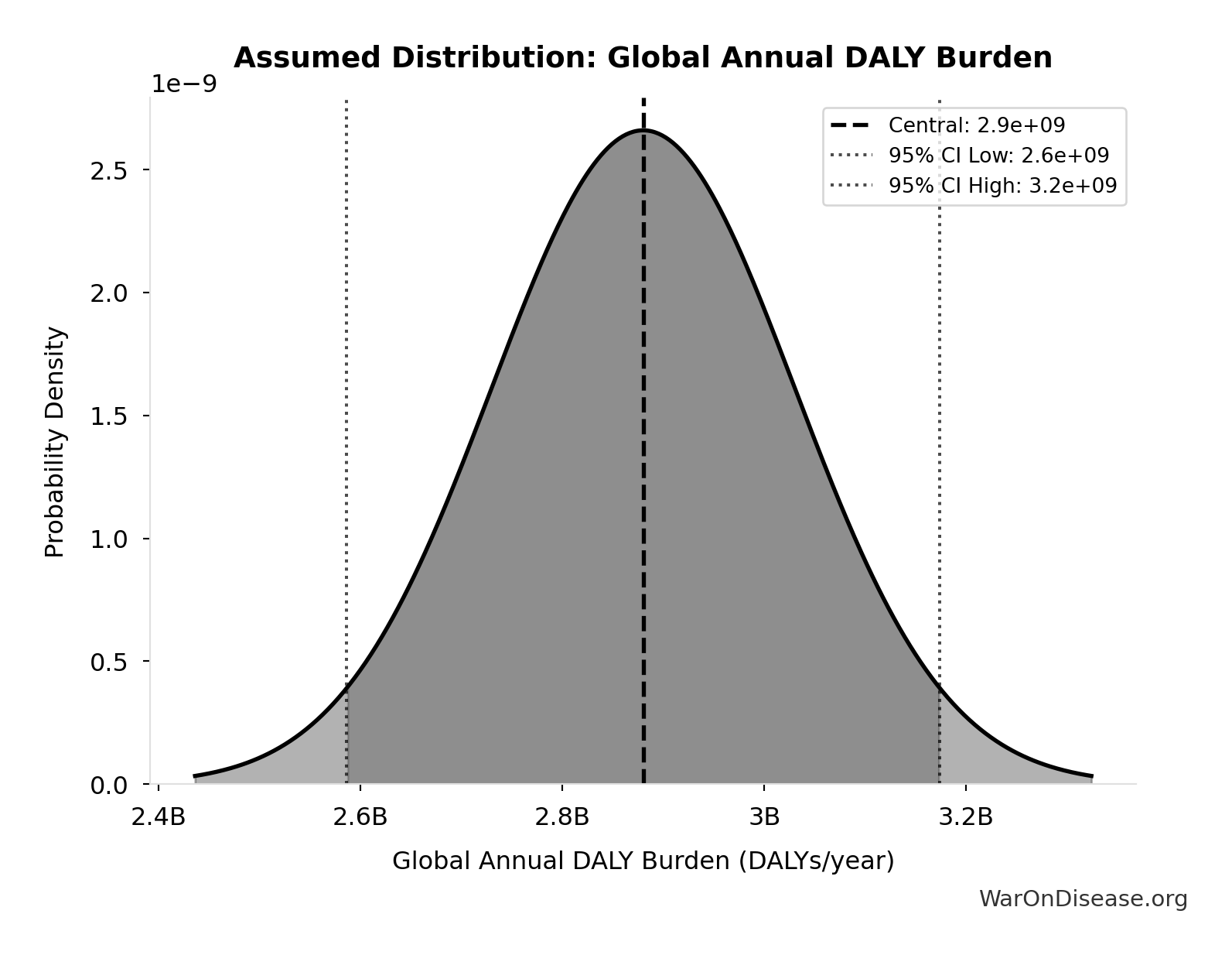
Global Annual DALY Burden: 2.88B DALYs/year
Global annual DALY burden from all diseases and injuries (WHO/IHME Global Burden of Disease 2021). Includes both YLL (years of life lost) and YLD (years lived with disability) from all causes.
Source:32
Uncertainty Range
Technical: Distribution: Normal (SE: 150M DALYs/year)
Input Distribution
This chart shows the assumed probability distribution for this parameter. The shaded region represents the 95% confidence interval where we expect the true value to fall.
✓ High confidence • 📊 Peer-reviewed
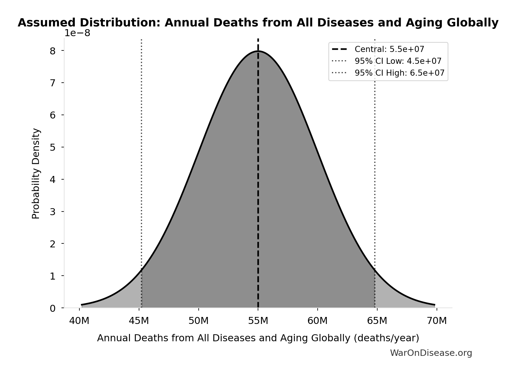
Annual Deaths from All Diseases and Aging Globally: 55.0M deaths/year
Annual deaths from all diseases and aging globally
Source:4
Uncertainty Range
Technical: Distribution: Normal (SE: 5.00M deaths/year)
Input Distribution
This chart shows the assumed probability distribution for this parameter. The shaded region represents the 95% confidence interval where we expect the true value to fall.
✓ High confidence
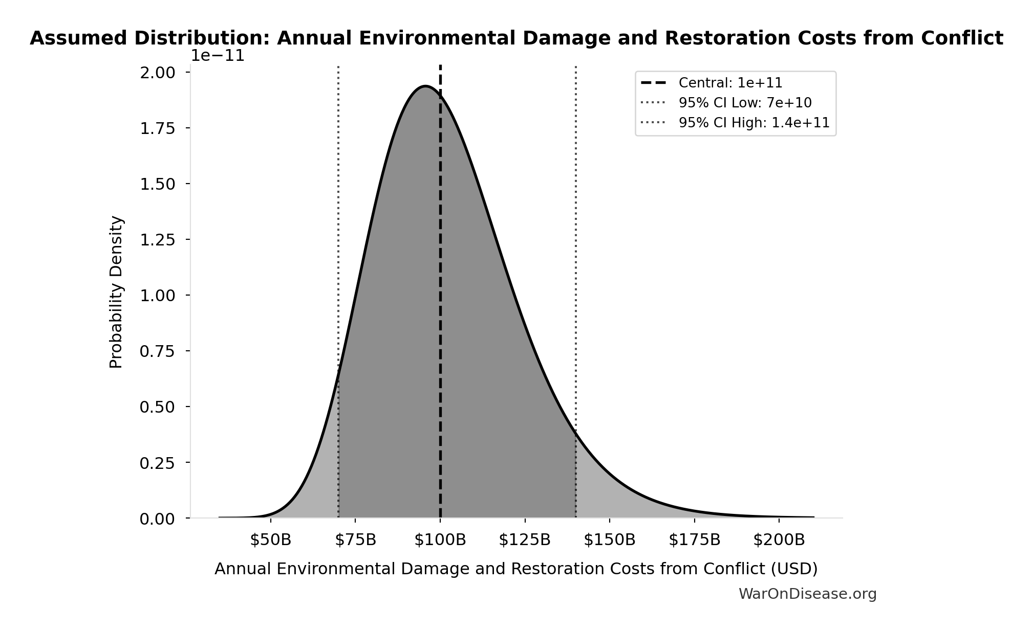
Annual Environmental Damage and Restoration Costs from Conflict: $100B
Annual environmental damage and restoration costs from conflict
Source:33
Uncertainty Range
Technical: 95% CI: [$70B, $140B] • Distribution: Lognormal
What this means: There’s significant uncertainty here. The true value likely falls between $70B and $140B (±35%). This represents a wide range that our Monte Carlo simulations account for when calculating overall uncertainty in the results.
The lognormal distribution means values can’t go negative and have a longer tail toward higher values (common for costs and populations).
Input Distribution
This chart shows the assumed probability distribution for this parameter. The shaded region represents the 95% confidence interval where we expect the true value to fall.
✓ High confidence
Annual Infrastructure Damage to Communications from Conflict: $298B
Annual infrastructure damage to communications from conflict
Source:33
Uncertainty Range
Technical: 95% CI: [$209B, $418B] • Distribution: Lognormal
What this means: There’s significant uncertainty here. The true value likely falls between $209B and $418B (±35%). This represents a wide range that our Monte Carlo simulations account for when calculating overall uncertainty in the results.
The lognormal distribution means values can’t go negative and have a longer tail toward higher values (common for costs and populations).
Input Distribution
This chart shows the assumed probability distribution for this parameter. The shaded region represents the 95% confidence interval where we expect the true value to fall.
✓ High confidence
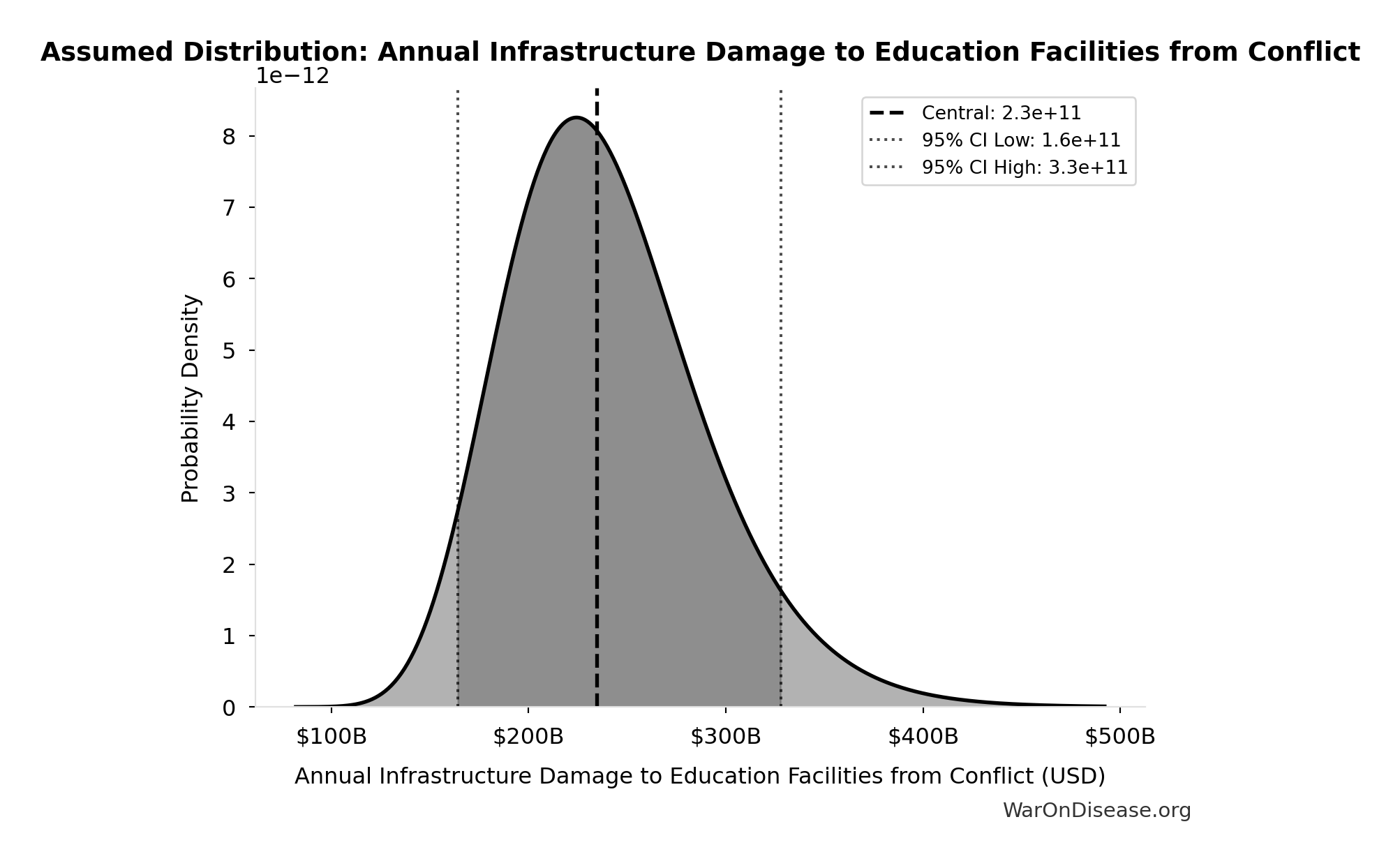
Annual Infrastructure Damage to Education Facilities from Conflict: $234B
Annual infrastructure damage to education facilities from conflict
Source:33
Uncertainty Range
Technical: 95% CI: [$164B, $328B] • Distribution: Lognormal
What this means: There’s significant uncertainty here. The true value likely falls between $164B and $328B (±35%). This represents a wide range that our Monte Carlo simulations account for when calculating overall uncertainty in the results.
The lognormal distribution means values can’t go negative and have a longer tail toward higher values (common for costs and populations).
Input Distribution
This chart shows the assumed probability distribution for this parameter. The shaded region represents the 95% confidence interval where we expect the true value to fall.
✓ High confidence
Annual Infrastructure Damage to Energy Systems from Conflict: $422B
Annual infrastructure damage to energy systems from conflict
Source:33
Uncertainty Range
Technical: 95% CI: [$295B, $590B] • Distribution: Lognormal
What this means: There’s significant uncertainty here. The true value likely falls between $295B and $590B (±35%). This represents a wide range that our Monte Carlo simulations account for when calculating overall uncertainty in the results.
The lognormal distribution means values can’t go negative and have a longer tail toward higher values (common for costs and populations).
Input Distribution
This chart shows the assumed probability distribution for this parameter. The shaded region represents the 95% confidence interval where we expect the true value to fall.
✓ High confidence
Annual Infrastructure Damage to Healthcare Facilities from Conflict: $166B
Annual infrastructure damage to healthcare facilities from conflict
Source:33
Uncertainty Range
Technical: 95% CI: [$116B, $232B] • Distribution: Lognormal
What this means: There’s significant uncertainty here. The true value likely falls between $116B and $232B (±35%). This represents a wide range that our Monte Carlo simulations account for when calculating overall uncertainty in the results.
The lognormal distribution means values can’t go negative and have a longer tail toward higher values (common for costs and populations).
Input Distribution
This chart shows the assumed probability distribution for this parameter. The shaded region represents the 95% confidence interval where we expect the true value to fall.
✓ High confidence
Annual Infrastructure Damage to Transportation from Conflict: $487B
Annual infrastructure damage to transportation from conflict
Source:33
Uncertainty Range
Technical: 95% CI: [$340B, $680B] • Distribution: Lognormal
What this means: There’s significant uncertainty here. The true value likely falls between $340B and $680B (±35%). This represents a wide range that our Monte Carlo simulations account for when calculating overall uncertainty in the results.
The lognormal distribution means values can’t go negative and have a longer tail toward higher values (common for costs and populations).
Input Distribution
This chart shows the assumed probability distribution for this parameter. The shaded region represents the 95% confidence interval where we expect the true value to fall.
✓ High confidence
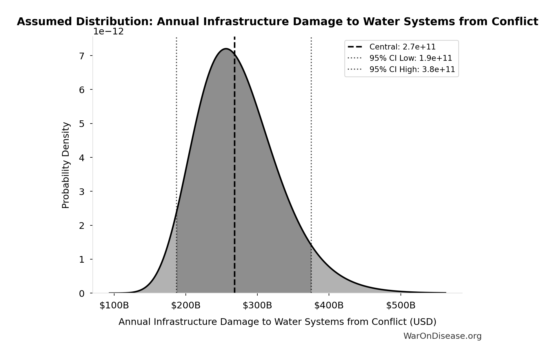
Annual Infrastructure Damage to Water Systems from Conflict: $268B
Annual infrastructure damage to water systems from conflict
Source:33
Uncertainty Range
Technical: 95% CI: [$187B, $375B] • Distribution: Lognormal
What this means: There’s significant uncertainty here. The true value likely falls between $187B and $375B (±35%). This represents a wide range that our Monte Carlo simulations account for when calculating overall uncertainty in the results.
The lognormal distribution means values can’t go negative and have a longer tail toward higher values (common for costs and populations).
Input Distribution
This chart shows the assumed probability distribution for this parameter. The shaded region represents the 95% confidence interval where we expect the true value to fall.
✓ High confidence
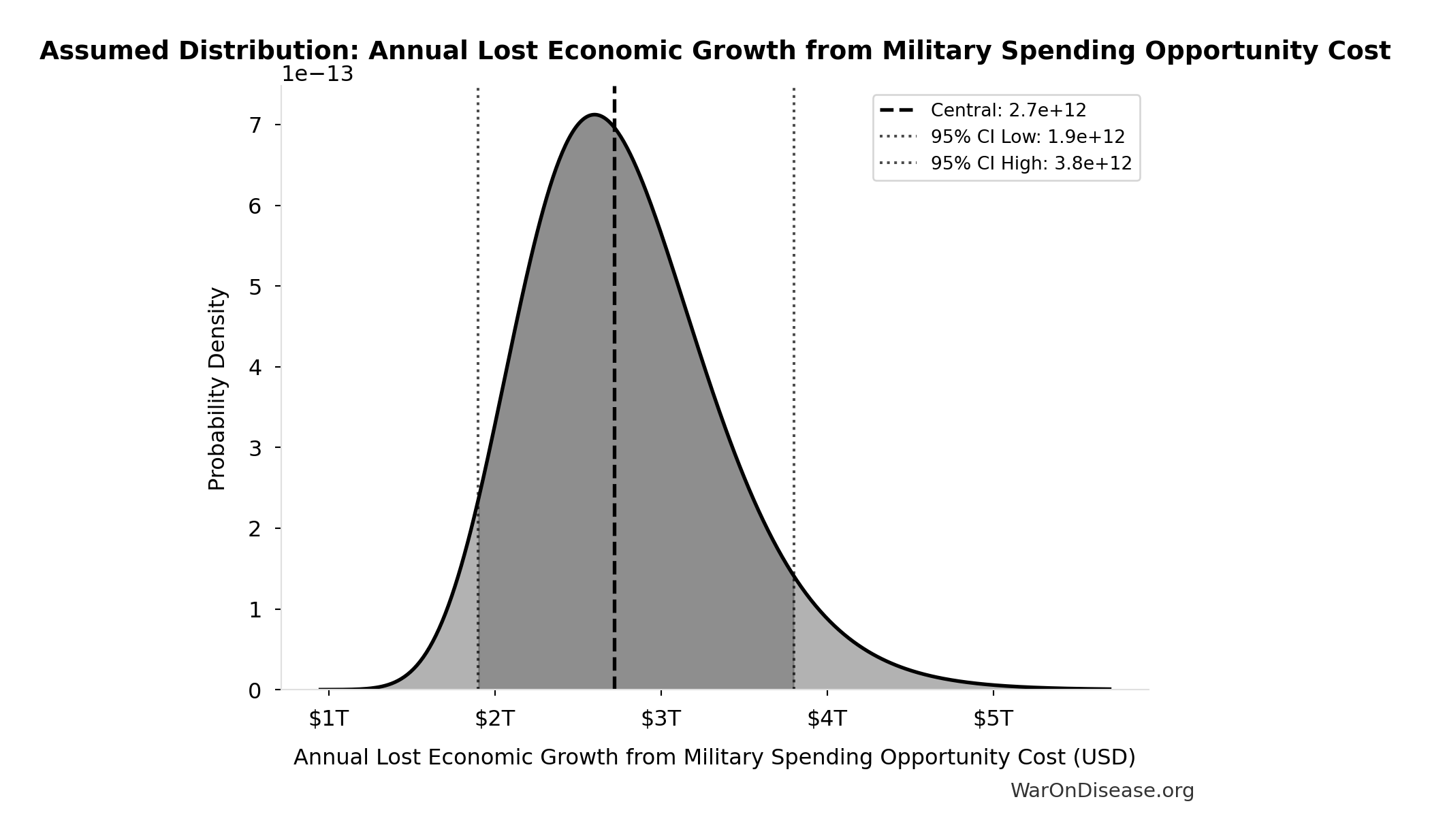
Annual Lost Economic Growth from Military Spending Opportunity Cost: $2.72T
Annual foregone economic output from military spending vs productive alternatives. This estimate implicitly captures fiscal multiplier differences (military ~0.6x vs healthcare ~4.3x GDP multiplier). Do not add separate GDP multiplier adjustment to avoid double-counting.
Source:35
Uncertainty Range
Technical: 95% CI: [$1.90T, $3.80T] • Distribution: Lognormal
What this means: There’s significant uncertainty here. The true value likely falls between $1.90T and $3.80T (±35%). This represents a wide range that our Monte Carlo simulations account for when calculating overall uncertainty in the results.
The lognormal distribution means values can’t go negative and have a longer tail toward higher values (common for costs and populations).
Input Distribution
This chart shows the assumed probability distribution for this parameter. The shaded region represents the 95% confidence interval where we expect the true value to fall.
✓ High confidence
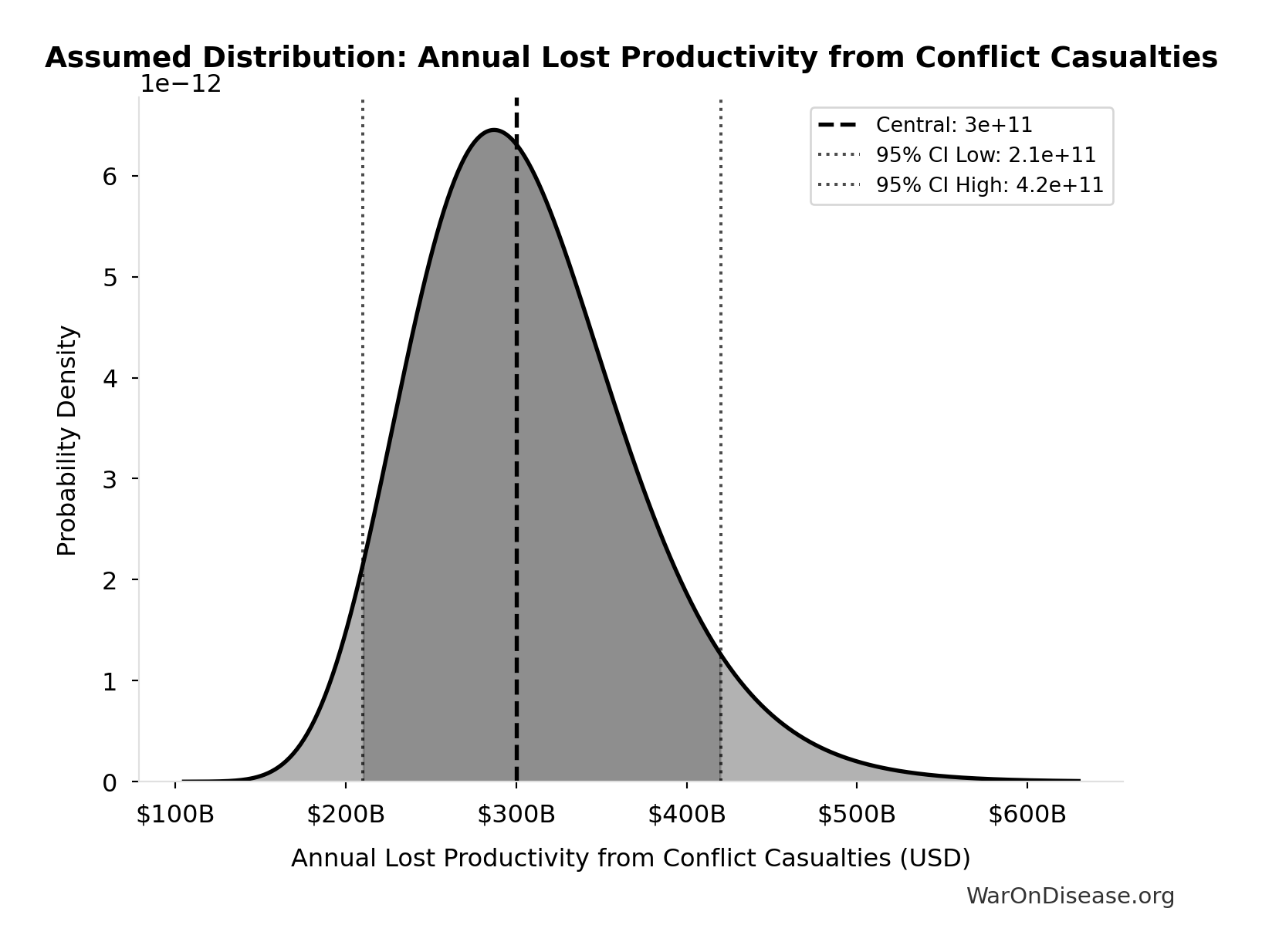
Annual Lost Productivity from Conflict Casualties: $300B
Annual lost productivity from conflict casualties
Source:36
Uncertainty Range
Technical: 95% CI: [$210B, $420B] • Distribution: Lognormal
What this means: There’s significant uncertainty here. The true value likely falls between $210B and $420B (±35%). This represents a wide range that our Monte Carlo simulations account for when calculating overall uncertainty in the results.
The lognormal distribution means values can’t go negative and have a longer tail toward higher values (common for costs and populations).
Input Distribution
This chart shows the assumed probability distribution for this parameter. The shaded region represents the 95% confidence interval where we expect the true value to fall.
✓ High confidence
Annual PTSD and Mental Health Costs from Conflict: $232B
Annual PTSD and mental health costs from conflict
Source:37
Uncertainty Range
Technical: 95% CI: [$162B, $325B] • Distribution: Lognormal
What this means: There’s significant uncertainty here. The true value likely falls between $162B and $325B (±35%). This represents a wide range that our Monte Carlo simulations account for when calculating overall uncertainty in the results.
The lognormal distribution means values can’t go negative and have a longer tail toward higher values (common for costs and populations).
Input Distribution
This chart shows the assumed probability distribution for this parameter. The shaded region represents the 95% confidence interval where we expect the true value to fall.
✓ High confidence
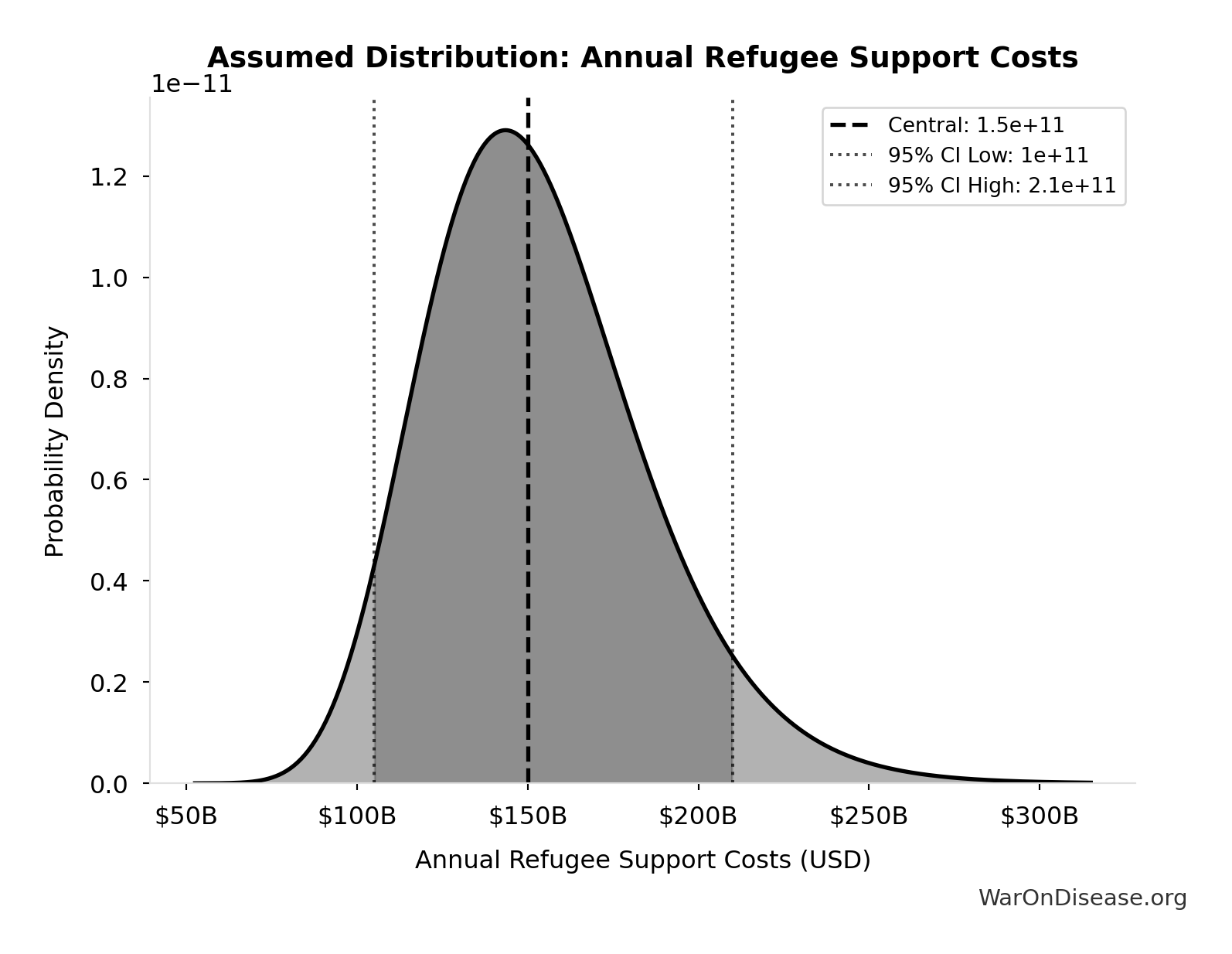
Annual Refugee Support Costs: $150B
Annual refugee support costs (108.4M refugees × $1,384/year)
Source:38
Uncertainty Range
Technical: 95% CI: [$105B, $210B] • Distribution: Lognormal
What this means: There’s significant uncertainty here. The true value likely falls between $105B and $210B (±35%). This represents a wide range that our Monte Carlo simulations account for when calculating overall uncertainty in the results.
The lognormal distribution means values can’t go negative and have a longer tail toward higher values (common for costs and populations).
Input Distribution
This chart shows the assumed probability distribution for this parameter. The shaded region represents the 95% confidence interval where we expect the true value to fall.
✓ High confidence
Annual Trade Disruption Costs from Currency Instability: $57.4B
Annual trade disruption costs from currency instability
Source:39
Uncertainty Range
Technical: 95% CI: [$40B, $80B] • Distribution: Lognormal
What this means: There’s significant uncertainty here. The true value likely falls between $40B and $80B (±35%). This represents a wide range that our Monte Carlo simulations account for when calculating overall uncertainty in the results.
The lognormal distribution means values can’t go negative and have a longer tail toward higher values (common for costs and populations).
Input Distribution
This chart shows the assumed probability distribution for this parameter. The shaded region represents the 95% confidence interval where we expect the true value to fall.
✓ High confidence
Annual Trade Disruption Costs from Energy Price Volatility: $125B
Annual trade disruption costs from energy price volatility
Source:39
Uncertainty Range
Technical: 95% CI: [$87B, $175B] • Distribution: Lognormal
What this means: There’s significant uncertainty here. The true value likely falls between $87B and $175B (±35%). This represents a wide range that our Monte Carlo simulations account for when calculating overall uncertainty in the results.
The lognormal distribution means values can’t go negative and have a longer tail toward higher values (common for costs and populations).
Input Distribution
This chart shows the assumed probability distribution for this parameter. The shaded region represents the 95% confidence interval where we expect the true value to fall.
✓ High confidence
Annual Trade Disruption Costs from Shipping Disruptions: $247B
Annual trade disruption costs from shipping disruptions
Source:39
Uncertainty Range
Technical: 95% CI: [$173B, $346B] • Distribution: Lognormal
What this means: There’s significant uncertainty here. The true value likely falls between $173B and $346B (±35%). This represents a wide range that our Monte Carlo simulations account for when calculating overall uncertainty in the results.
The lognormal distribution means values can’t go negative and have a longer tail toward higher values (common for costs and populations).
Input Distribution
This chart shows the assumed probability distribution for this parameter. The shaded region represents the 95% confidence interval where we expect the true value to fall.
✓ High confidence
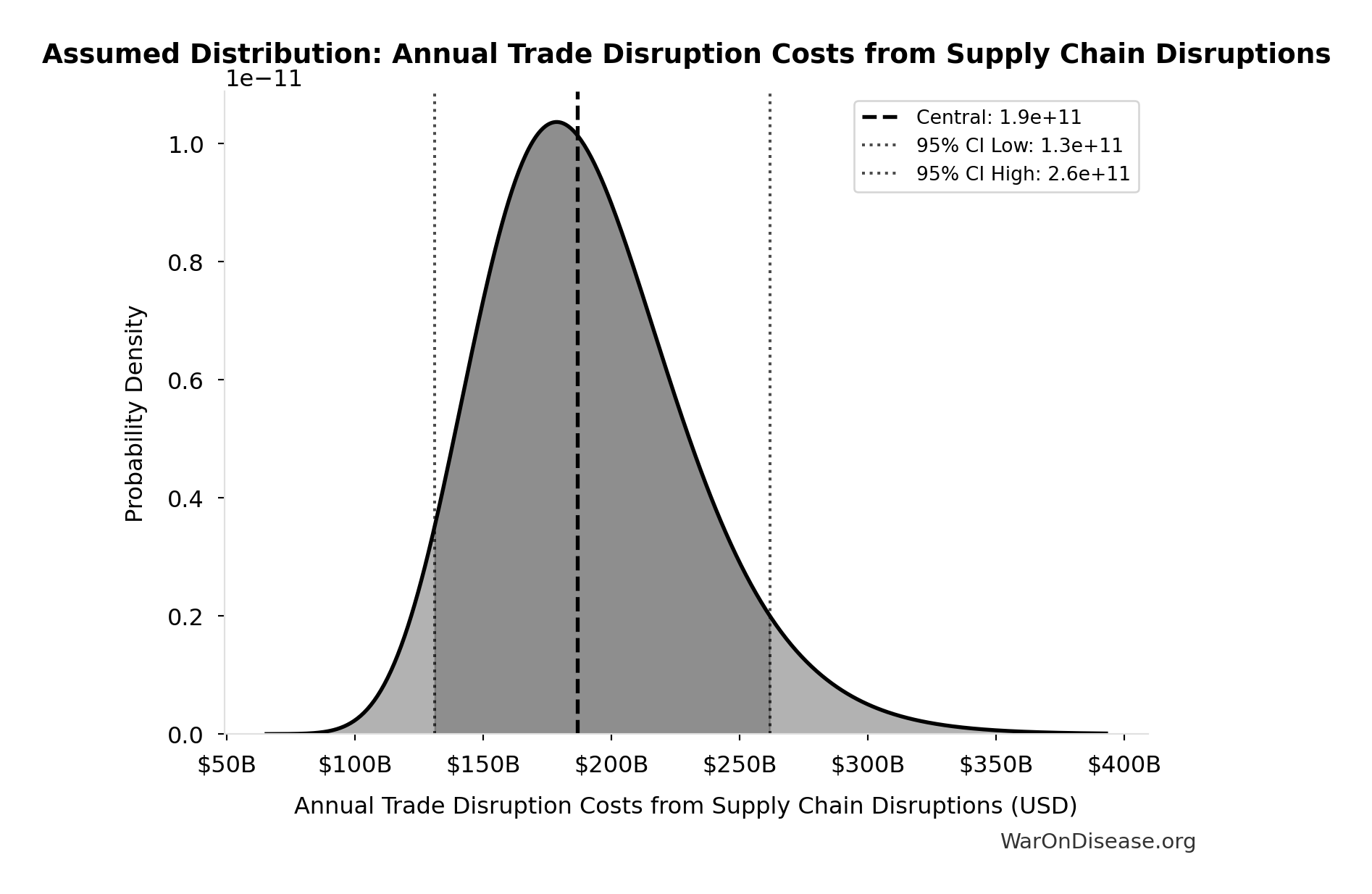
Annual Trade Disruption Costs from Supply Chain Disruptions: $187B
Annual trade disruption costs from supply chain disruptions
Source:39
Uncertainty Range
Technical: 95% CI: [$131B, $262B] • Distribution: Lognormal
What this means: There’s significant uncertainty here. The true value likely falls between $131B and $262B (±35%). This represents a wide range that our Monte Carlo simulations account for when calculating overall uncertainty in the results.
The lognormal distribution means values can’t go negative and have a longer tail toward higher values (common for costs and populations).
Input Distribution
This chart shows the assumed probability distribution for this parameter. The shaded region represents the 95% confidence interval where we expect the true value to fall.
✓ High confidence
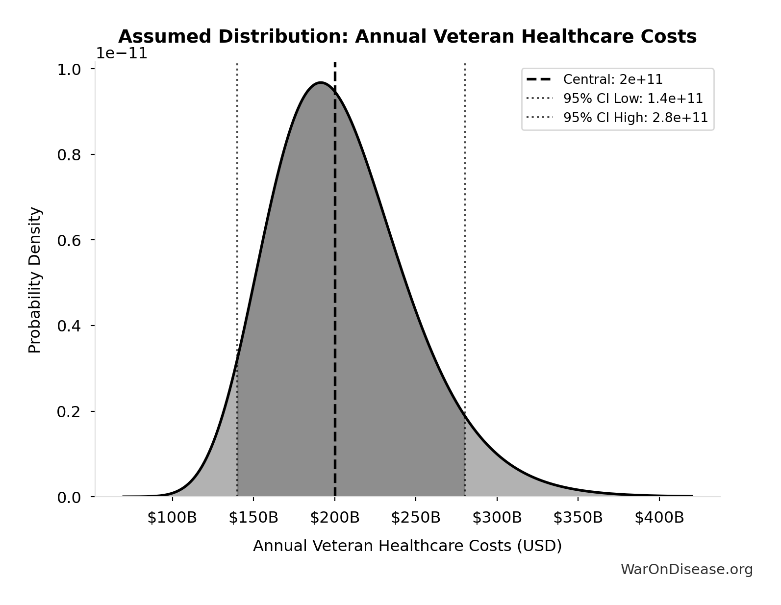
Annual Veteran Healthcare Costs: $200B
Annual veteran healthcare costs (20-year projected)
Source:40
Uncertainty Range
Technical: 95% CI: [$140B, $280B] • Distribution: Lognormal
What this means: There’s significant uncertainty here. The true value likely falls between $140B and $280B (±35%). This represents a wide range that our Monte Carlo simulations account for when calculating overall uncertainty in the results.
The lognormal distribution means values can’t go negative and have a longer tail toward higher values (common for costs and populations).
Input Distribution
This chart shows the assumed probability distribution for this parameter. The shaded region represents the 95% confidence interval where we expect the true value to fall.
✓ High confidence
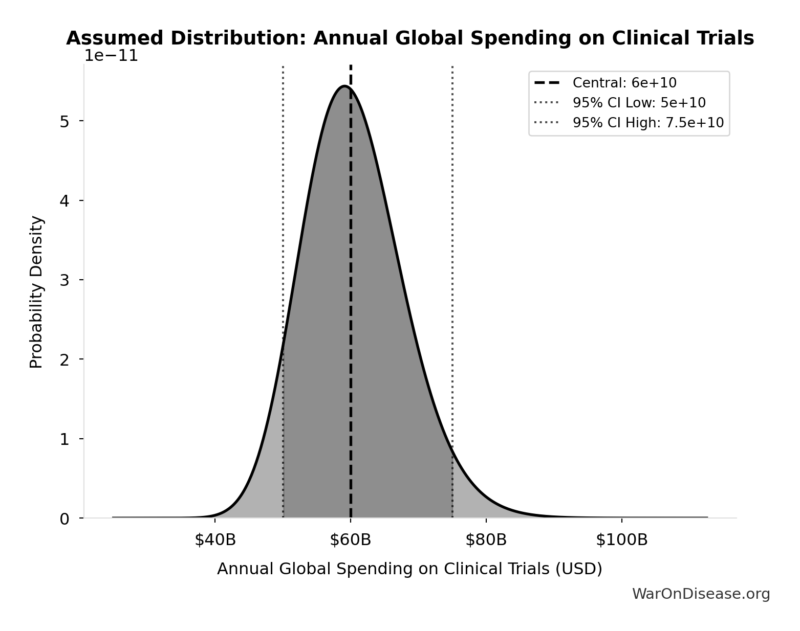
Annual Global Spending on Clinical Trials: $60B
Annual global spending on clinical trials (Industry: $45-60B + Government: $3-6B + Nonprofits: $2-5B). Conservative estimate using 15-20% of $300B total pharma R&D, not inflated market size projections.
Source:42
Uncertainty Range
Technical: 95% CI: [$50B, $75B] • Distribution: Lognormal (SE: $10B)
What this means: This estimate has moderate uncertainty. The true value likely falls between $50B and $75B (±21%). This represents a reasonable range that our Monte Carlo simulations account for when calculating overall uncertainty in the results.
The lognormal distribution means values can’t go negative and have a longer tail toward higher values (common for costs and populations).
Input Distribution
This chart shows the assumed probability distribution for this parameter. The shaded region represents the 95% confidence interval where we expect the true value to fall.
✓ High confidence
Global Household Wealth: $454T
Global Military Spending in 2024: $2.72T
Global military spending in 2024
Source:48
Uncertainty Range
Technical: Distribution: Fixed
✓ High confidence
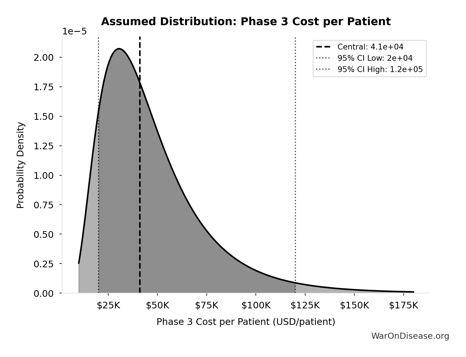
Phase 3 Cost per Patient: $41K
Phase 3 cost per patient (median from FDA study)
Source:101
Uncertainty Range
Technical: 95% CI: [$20K, $120K] • Distribution: Lognormal
What this means: This estimate is highly uncertain. The true value likely falls between $20K and $120K (±122%). This represents a very wide range that our Monte Carlo simulations account for when calculating overall uncertainty in the results.
The lognormal distribution means values can’t go negative and have a longer tail toward higher values (common for costs and populations).
Input Distribution
This chart shows the assumed probability distribution for this parameter. The shaded region represents the 95% confidence interval where we expect the true value to fall.
✓ High confidence
Value of Statistical Life: $10M
Value of Statistical Life (conservative estimate)
Source:127
Uncertainty Range
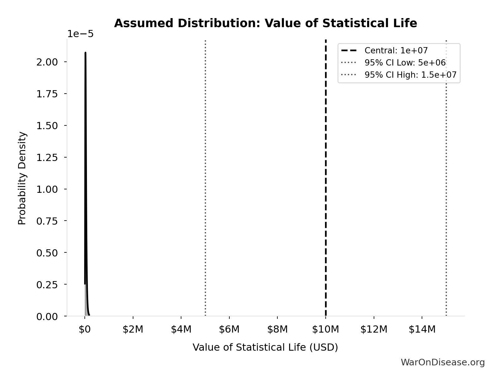
Technical: 95% CI: [$5M, $15M] • Distribution: Gamma (SE: $3M)
What this means: There’s significant uncertainty here. The true value likely falls between $5M and $15M (±50%). This represents a wide range that our Monte Carlo simulations account for when calculating overall uncertainty in the results.
The gamma distribution means values follow a specific statistical pattern.
Input Distribution
This chart shows the assumed probability distribution for this parameter. The shaded region represents the 95% confidence interval where we expect the true value to fall.
✓ High confidence
Core Definitions
Fundamental parameters and constants used throughout the analysis.
Concentrated Interest Sector Market Cap: $5T
Estimated combined market capitalization of concentrated interest opposition (defense, fossil fuel, etc.)
Core definition
IAB Mechanism Annual Cost (High Estimate): $750M
Estimated annual cost of the IAB mechanism (high-end estimate including regulatory defense)
Uncertainty Range
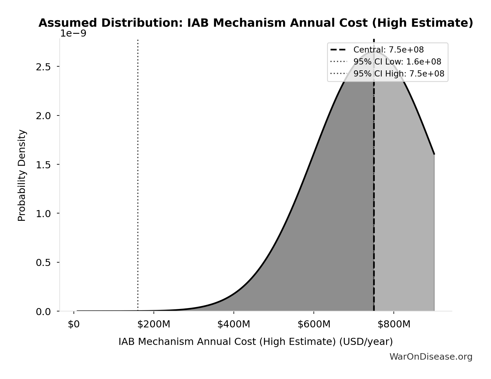
Technical: 95% CI: [$160M, $750M]
What this means: There’s significant uncertainty here. The true value likely falls between $160M and $750M (±39%). This represents a wide range that our Monte Carlo simulations account for when calculating overall uncertainty in the results.
Input Distribution
This chart shows the assumed probability distribution for this parameter. The shaded region represents the 95% confidence interval where we expect the true value to fall.
Core definition
IAB Political Incentive Funding Percentage: 10%
Percentage of treaty funding allocated to Incentive Alignment Bond mechanism for political incentives (independent expenditures/PACs, post-office fellowships, Public Good Score infrastructure)
Uncertainty Range
Technical: Distribution: Fixed
Core definition
Political Lobbying Campaign: Direct Lobbying, Super Pacs, Opposition Research, Staff, Legal/Compliance: $650M
Political lobbying campaign: direct lobbying (US/EU/G20), Super PACs, opposition research, staff, legal/compliance. Budget exceeds combined pharma ($300M/year) and military-industrial complex ($150M/year) lobbying to ensure competitive positioning. Referendum relies on grassroots mobilization and earned media, while lobbying requires matching or exceeding opposition spending for political viability.
Uncertainty Range
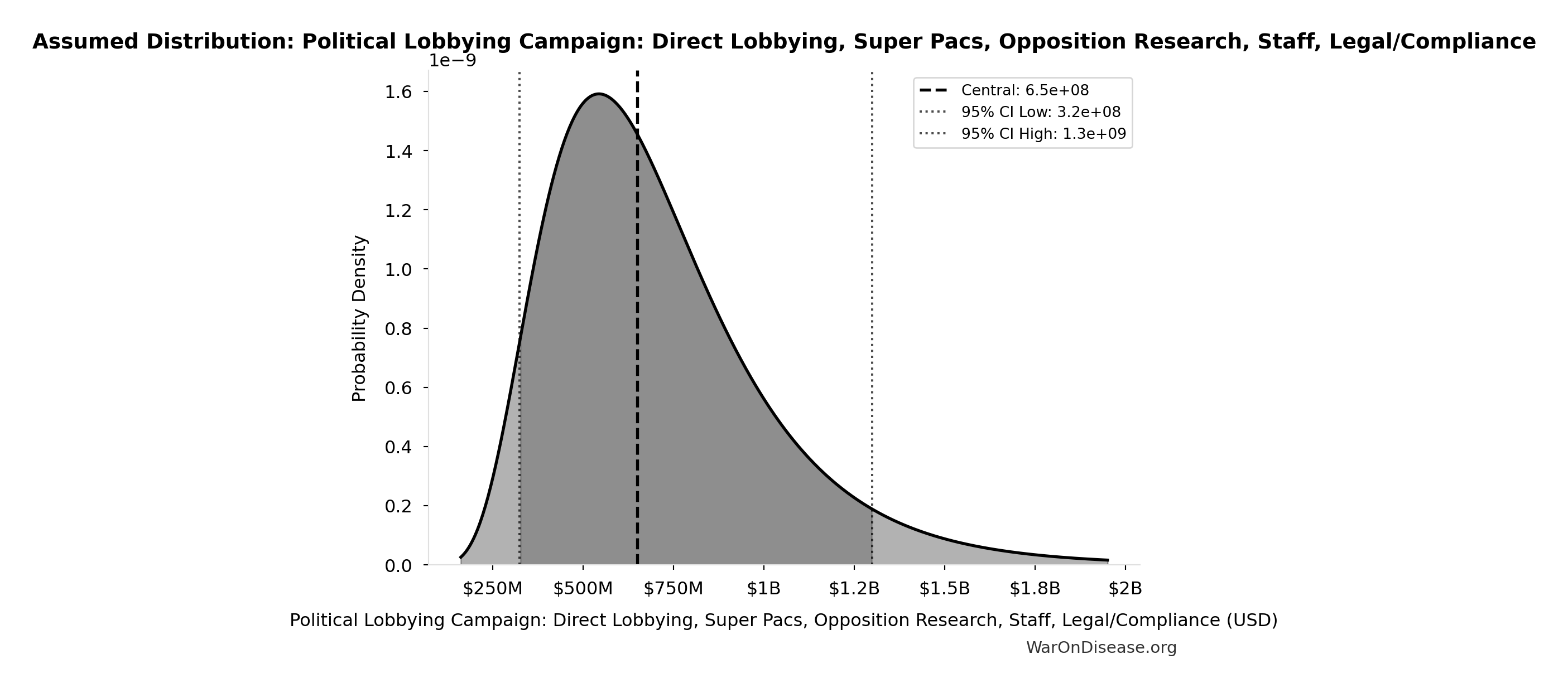
Technical: 95% CI: [$325M, $1.30B] • Distribution: Lognormal
What this means: This estimate is highly uncertain. The true value likely falls between $325M and $1.30B (±75%). This represents a very wide range that our Monte Carlo simulations account for when calculating overall uncertainty in the results.
The lognormal distribution means values can’t go negative and have a longer tail toward higher values (common for costs and populations).
Input Distribution
This chart shows the assumed probability distribution for this parameter. The shaded region represents the 95% confidence interval where we expect the true value to fall.
Core definition
Reserve Fund / Contingency Buffer: $100M
Reserve fund / contingency buffer (10% of total campaign cost). Using industry standard 10% for complex campaigns with potential for unforeseen legal challenges, opposition response, or regulatory delays. Conservative lower bound of $20M (2%) reflects transparent budget allocation and predictable referendum/lobbying costs.
Uncertainty Range
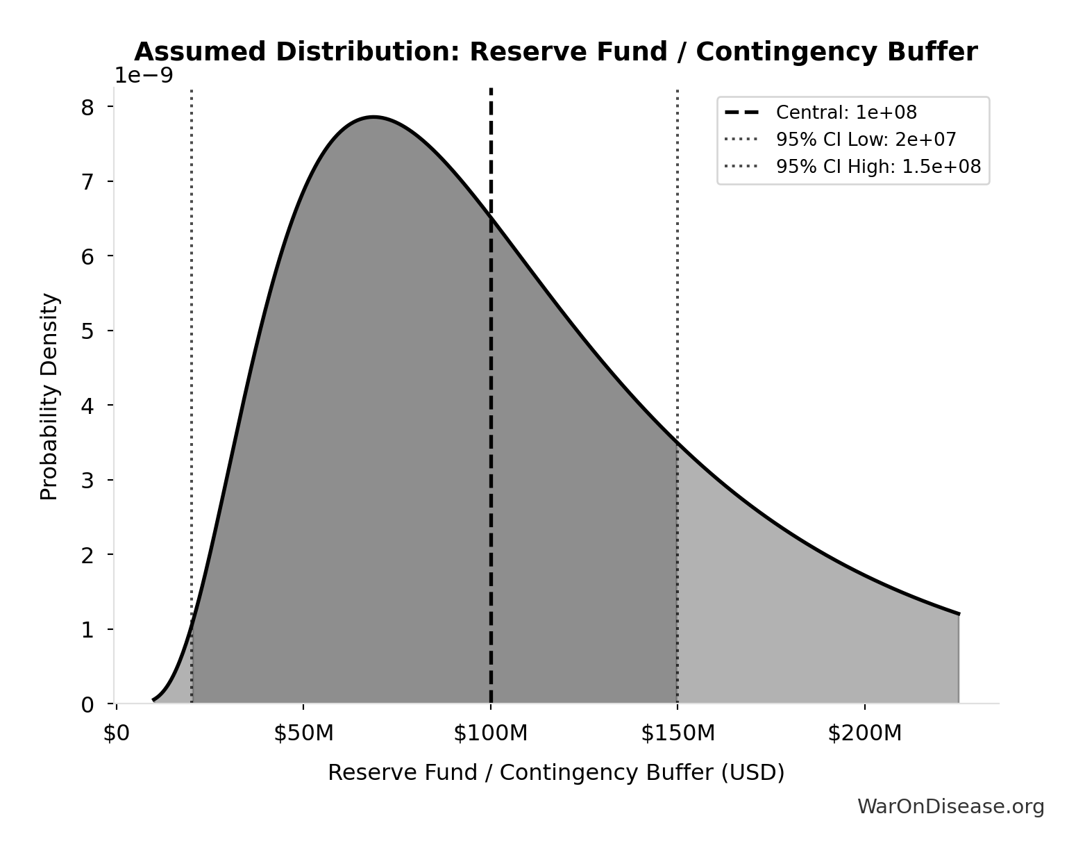
Technical: 95% CI: [$20M, $150M] • Distribution: Lognormal
What this means: This estimate is highly uncertain. The true value likely falls between $20M and $150M (±65%). This represents a very wide range that our Monte Carlo simulations account for when calculating overall uncertainty in the results.
The lognormal distribution means values can’t go negative and have a longer tail toward higher values (common for costs and populations).
Input Distribution
This chart shows the assumed probability distribution for this parameter. The shaded region represents the 95% confidence interval where we expect the true value to fall.
Core definition
1% Reduction in Military Spending/War Costs from Treaty: 1%
1% reduction in military spending/war costs from treaty
Uncertainty Range
Technical: Distribution: Fixed
Core definition
Percentage of Captured Dividend Funding VICTORY Incentive Alignment Bonds: 10%
Percentage of captured dividend funding VICTORY Incentive Alignment Bonds (10%)
Uncertainty Range
Technical: Distribution: Fixed
Core definition
